Understanding Independence and Bayes’ Rule
Learn how Bayes’ Theorem works, when to apply it, and how it connects to independence and conditional probability. This post breaks down key concepts with clear examples and practical relevance in real-world applications like spam detection and medical testing.
Understanding uncertainty is at the heart of statistics — and Bayes’ Rule is one of the most powerful tools to deal with it. This post will show you how Bayes’ Theorem helps us update probabilities with new information, and how it connects to independence, conditional probability, and real-world reasoning — from medical diagnoses to machine learning models. —
📚 This post is part of the "Intro to Statistics" series
🔙 Previously: Making Sense of Union, Tables, and Conditional Thinking
🔗 What Is Independence?
Two events are independent when the occurrence of one doesn’t affect the probability of the other.
📌 Mathematically:
Any of the following implies independence:
\[ P(A \mid B) = P(A) \] \[ P(B \mid A) = P(B) \] \[ P(A \cap B) = P(A) \cdot P(B) \]
If any of these holds, the events are independent.
🔄 Independence vs Disjoint
| Concept | Description |
|---|---|
| Disjoint (Mutually Exclusive) | Events can’t both happen. \( P(A \cap B) = 0 \) |
| Independent | One event doesn’t affect the other’s probability |
✅ Key Insight:
- If A and B are disjoint, then \( P(A \cap B) = 0 \)
- But that contradicts \( P(A) \cdot P(B) > 0 \) — so:
Disjoint events are always dependent.
Independent events are never disjoint (unless one has probability 0).
🧪 Example: Email Spam Detection
Suppose:
- 40% of all emails are spam → \( P(S) = 0.4 \)
- 80% of spam emails contain the word “free” → \( P(F \mid S) = 0.8 \)
- 10% of non-spam emails contain “free” → \( P(F \mid \bar{S}) = 0.1 \)
🌳 Build a Decision Tree
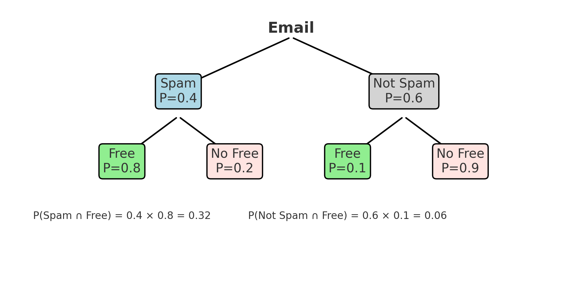 Figure: Tree diagram showing all outcomes for Spam vs Free
We can calculate all joint probabilities:
- \( P(S \cap F) = 0.4 \cdot 0.8 = 0.32 \)
- \( P(\bar{S} \cap F) = 0.6 \cdot 0.1 = 0.06 \)
- \( P(F) = 0.32 + 0.06 = 0.38 \)
📘 Bayes’ Theorem
Now, we want:
If I see “free” in an email, what’s the probability it’s spam?
📌 Formula:
\[ P(S \mid F) = \frac{P(S \cap F)}{P(F)} = \frac{0.32}{0.38} \approx 0.842 \]
🧠 Understanding Bayes’ Rule: Components
| Term | Meaning |
|---|---|
| Prior | What you believe before seeing the evidence → \( P(S) = 0.4 \) |
| Likelihood | Probability of the evidence given the hypothesis → \( P(F \mid S) \) |
| Evidence | Total probability of seeing “free” → \( P(F) = 0.38 \) |
| Posterior | Updated belief → \( P(S \mid F) = 0.842 \) |
🧠 Bayes’ Theorem in Action: Two Real-World Examples
📚 Example 1: Student Cheating Detection
A teacher knows that only 2% of students cheat on exams.
She uses a plagiarism detector that:
- Correctly identifies cheaters 90% of the time
- Wrongly flags innocent students 5% of the time
Now, a student gets flagged. What are the chances they actually cheated?
Let:
- \( C \): student cheated
- \( P \): student flagged
We know:
- \( P(C) = 0.02 \), \( P(\bar{C}) = 0.98 \)
- \( P(P \mid C) = 0.90 \)
- \( P(P \mid \bar{C}) = 0.05 \)
✏️ Bayes’ Theorem:
\[ P(C \mid P) = \frac{P(P \mid C) \cdot P(C)}{P(P \mid C) \cdot P(C) + P(P \mid \bar{C}) \cdot P(\bar{C})} \]
🔍 Interpretation:
- Numerator = Likelihood × Prior = \( 0.90 \cdot 0.02 = 0.018 \)
→ This is the joint probability of being a cheater and being flagged - Denominator = Total probability of being flagged
→ Includes both cheaters and non-cheaters who were flagged: \[ = 0.018 + (0.05 \cdot 0.98) = 0.018 + 0.049 = 0.067 \]
✅ Final Answer:
\[ P(C \mid P) = \frac{0.018}{0.067} \approx 0.268 \]
Even if flagged, there’s only a ~26.8% chance the student actually cheated.
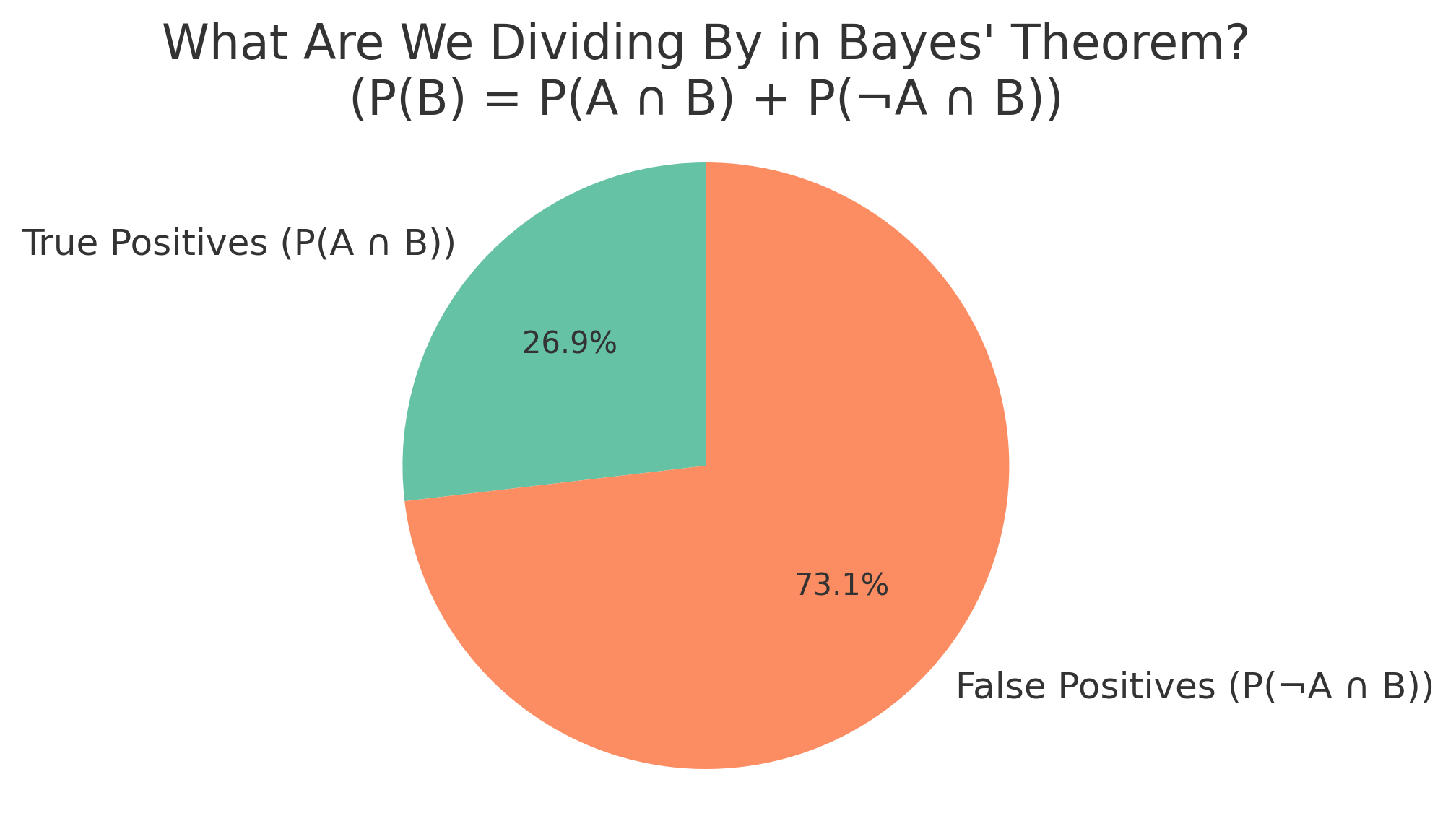 Figure: True vs False Positives that make up the total evidence (P(Flagged))
💊 Example 2: Random Drug Testing at Work
A company screens employees for a rare performance-enhancing drug.
- Only 1 in 1,000 uses it → \( P(D) = 0.001 \)
- The test is 99% accurate:
- \( P(+ \mid D) = 0.99 \)
- \( P(+ \mid \bar{D}) = 0.01 \)
An employee tests positive. What’s the probability they actually use the drug?
✏️ Bayes’ Theorem:
\[ P(D \mid +) = \frac{P(+ \mid D) \cdot P(D)}{P(+ \mid D) \cdot P(D) + P(+ \mid \bar{D}) \cdot P(\bar{D})} \]
🔍 Interpretation:
- Numerator = Likelihood × Prior = \( 0.99 \cdot 0.001 = 0.00099 \)
→ This is the joint probability of actually using the drug and testing positive - Denominator = Total probability of testing positive: \[ = 0.00099 + (0.01 \cdot 0.999) = 0.00099 + 0.00999 = 0.01098 \]
✅ Final Answer:
\[ P(D \mid +) = \frac{0.00099}{0.01098} \approx 0.09 \]
Despite a positive result, there’s only a ~9% chance the employee actually uses the drug — because the condition is rare, and false positives dominate the denominator.
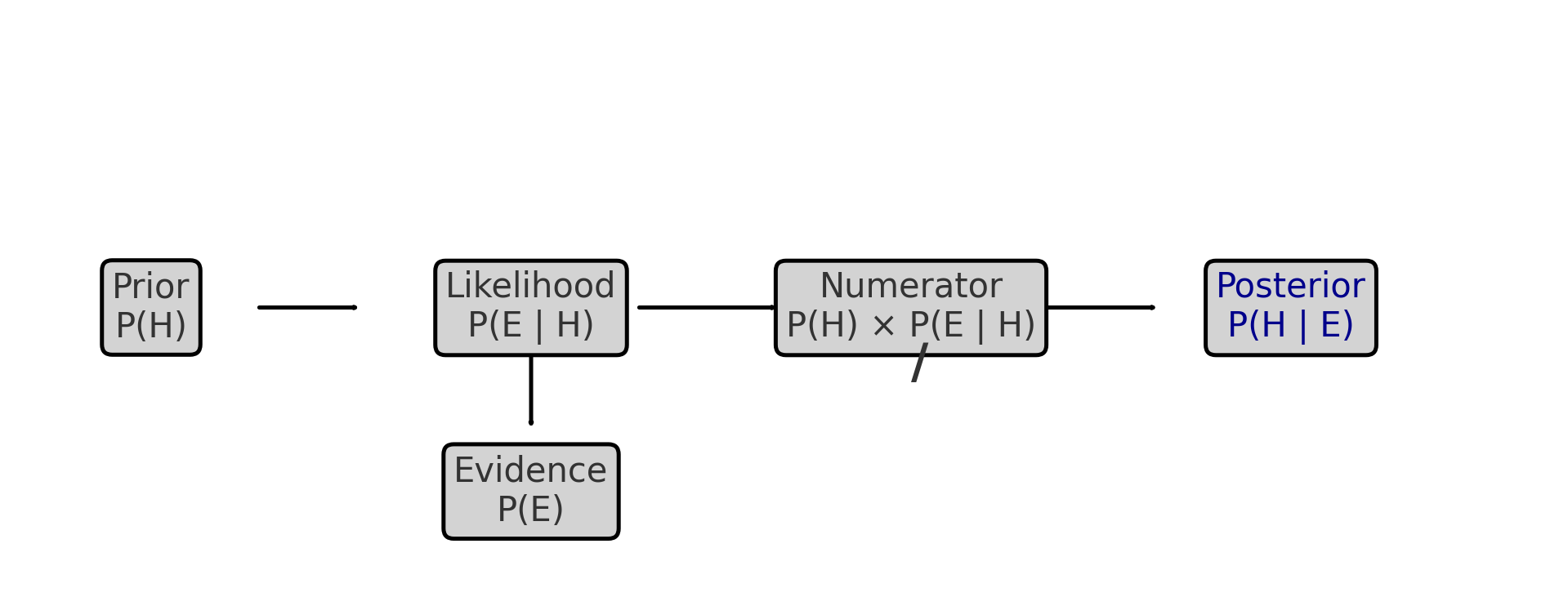 Figure: Flow of belief update — from prior and likelihood to posterior
🧠 Level Up: Mastering Bayes — What’s Really Going On?
Bayes’ Theorem might look like a formula — but it’s actually a way of reversing conditional logic.
- 🎯 The numerator is the probability that both the hypothesis and evidence are true (joint probability).
- 🧪 The denominator is the total probability of the observed evidence — from all possible sources.
So Bayes’ Theorem simply asks:
If this result just happened, how likely was it caused by what I suspected?
🧠 You’re updating your belief (the prior) based on what you just saw (the evidence), and how likely that evidence is under each possible explanation (likelihood).
Bayes is not just math — it’s decision logic under uncertainty.
✅ Best Practices for Bayes’ Rule
- Understand the difference between prior, likelihood, and posterior before applying the formula.
- Use tree diagrams or tables to break down problems clearly.
- Double-check that your events are independent when assuming so.
- Always compute total probability in the denominator correctly.
⚠️ Common Pitfalls
- ❌ Confusing P(A | B) with P(B | A).
- ❌ Ignoring base rates (priors), especially when they are very small.
- ❌ Mislabeling dependent events as independent.
- ❌ Forgetting to normalize with the full evidence probability in the denominator.
📌 Try It Yourself: Independence & Bayes
Q1: If \( P(A \mid B) = P(A) \), what does this imply?
💡 Show Answer
✅ Independence — it means that knowing B occurred does not change the probability of A.
So A and B are independent events.
Q2: Can disjoint events be independent?
💡 Show Answer
❌ No — disjoint events cannot both happen together, so the occurrence of one means the other definitely didn’t happen.
That makes them dependent by definition.
Q3: What is the formula for Bayes’ Theorem?
💡 Show Answer
✅ Bayes’ Rule:
P(A | B) = [P(B | A) × P(A)] ÷ P(B)
It allows us to reverse conditional probabilities based on observed evidence.
Bonus: Why is Bayes’ Rule so powerful in real-world applications?
💡 Show Answer
✅ It helps update probabilities when new evidence appears.
Whether in medical tests, spam filters, or AI predictions, Bayes’ Rule allows smart decision-making based on prior knowledge.
🧠 Summary
| Concept | Meaning |
|---|---|
| Independence | One event does not affect the other |
| Disjoint | Events can’t happen together |
| Joint from Marginal | Only possible if events are independent |
| Bayes’ Rule | Updates belief with new data |
| Prior | Initial belief |
| Likelihood | How likely the data is under a hypothesis |
| Posterior | Updated probability |
| Evidence | Total probability of the observed condition |
✅ Up Next
Next, we’ll dive into probability distributions and how cumulative distributions help us model real-world events over time.
Stay tuned!
📺 Explore the Channel

🎥 Hoda Osama AI
Learn statistics and machine learning concepts step by step with visuals and real examples.
💬 Got a Question?
Leave a comment or open an issue on GitHub — I love connecting with other learners and builders. 🔁