Confidence Interval for a Known Population Standard Deviation

🎯 Goal: Estimating a Population Mean with Known Standard Deviation

In statistics, estimating the true population mean (\( \mu \)) using a sample mean (\( \bar{x} \)) is a core task in inferential analysis.

This post explains how to calculate a Confidence Interval when the population standard deviation (\( \sigma \)) is known — a scenario where we use the Z-distribution instead of the T-distribution.

---

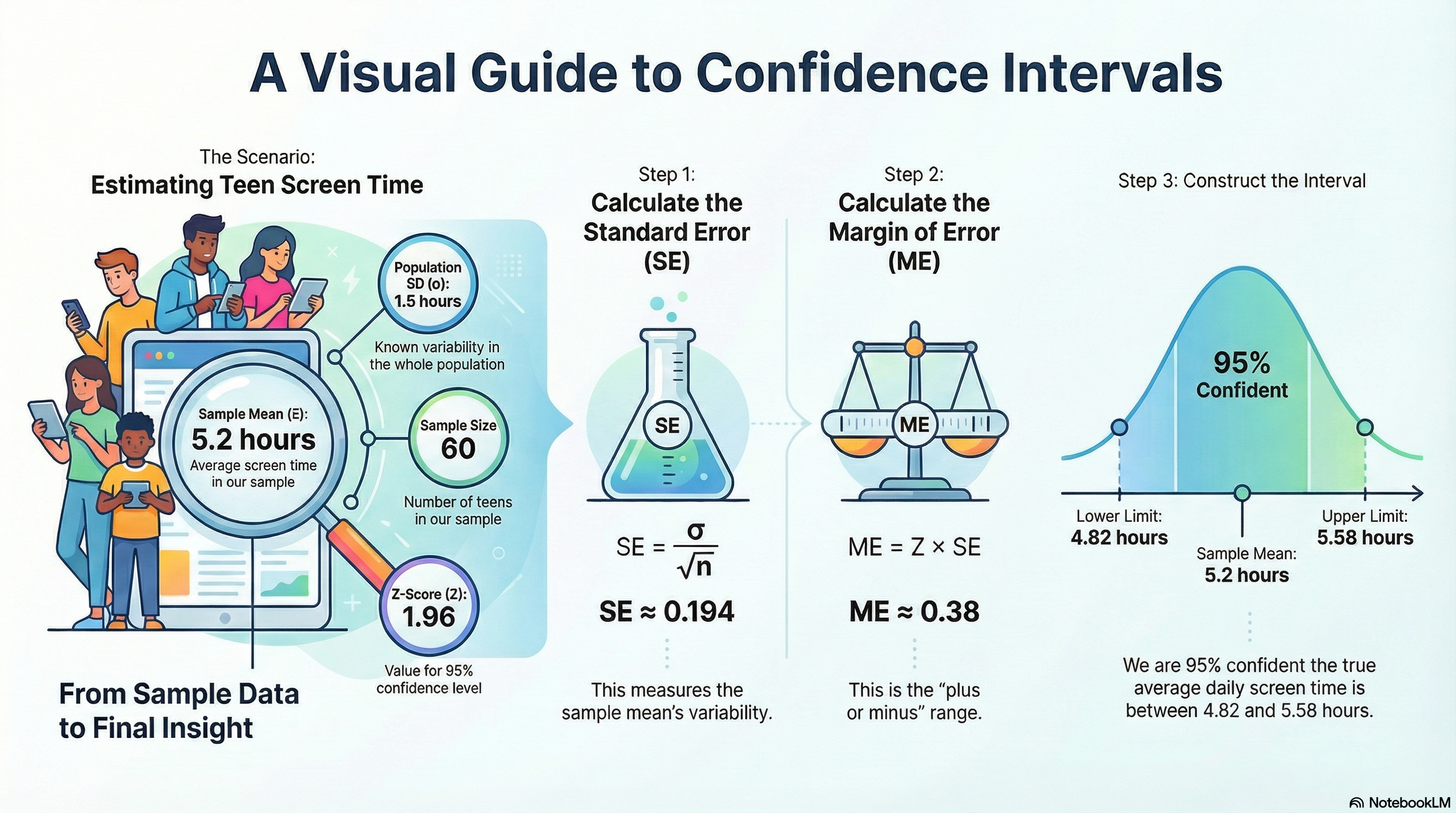
📱 Real-World Case: Teenagers’ Daily Screen Time

Imagine you’re analyzing national survey data on teenagers’ daily screen time (phones, laptops, TV).

A previous nationwide health report tells us the standard deviation of screen time across the full population of teens is \( \sigma = 1.5 \) hours.

You’re working with a random sample of 60 teenagers, and you find that:

• Sample Mean: \( \bar{x} = 5.2 \) hours/day
• Known Population SD: \( \sigma = 1.5 \) hours
• Sample Size: \( n = 60 \)
• Confidence Level: 95% (Z = 1.96)

---

📊 Step-by-Step: Building the Confidence Interval

🔹 Step 1: Calculate the Standard Error

\[ SE = \frac{\sigma}{\sqrt{n}} = \frac{1.5}{\sqrt{60}} \approx 0.1936 \]

---

🔹 Step 2: Calculate the Margin of Error

\[ ME = Z \times SE = 1.96 \times 0.1936 \approx 0.3794 \]

---

🔹 Step 3: Construct the Confidence Interval

\[ \bar{x} \pm ME = 5.2 \pm 0.3794 \]

• Lower Bound: \( 5.2 - 0.3794 = 4.82 \)
• Upper Bound: \( 5.2 + 0.3794 = 5.58 \)

✅ Conclusion: We are 95% confident that the true average screen time among all teenagers is between 4.82 and 5.58 hours per day.

---

---

🧠 Level Up: Why This Matters for Machine Learning

In ML, you’re often making predictions on unseen populations. Whether it’s user behavior, healthcare diagnostics, or marketing trends — understanding confidence intervals helps model generalization.

• 🔍 Precision vs Confidence: A wider interval gives more confidence but less precision. A narrower interval is more precise but riskier.
• 🎯 If you want a narrower range, increase the sample size to reduce standard error.

---

🐍 Python in Practice: CI with Known Standard Deviation

import numpy as np
import scipy.stats as stats

# Given data
sample_mean = 5.2
sigma = 1.5
n = 60
z = 1.96

# Standard Error
se = sigma / np.sqrt(n)

# Margin of Error
me = z * se

# Confidence Interval
ci_lower = sample_mean - me
ci_upper = sample_mean + me

print(f"95% CI: ({ci_lower:.2f}, {ci_upper:.2f})")

---

📏 Quick Reference: Steps to Calculate

1. ✅ Collect your data
   • Sample size \( n \)
   • Sample mean \( \bar{x} \)
   • Known population standard deviation \( \sigma \)
2. ✅ Choose your confidence level
   • Common choices:
     • 90% → \( Z = 1.645 \)
     • 95% → \( Z = 1.96 \)
     • 99% → \( Z = 2.576 \)

3. ✅ Calculate the Standard Error (SE)
   \[ SE = \frac{\sigma}{\sqrt{n}} \]

4. ✅ Calculate the Margin of Error (ME)
   \[ ME = Z \times SE \]

5. ✅ Construct the Confidence Interval
   \[ \bar{x} \pm ME \]
   • Lower bound: \( \bar{x} - ME \)
   • Upper bound: \( \bar{x} + ME \)

---

✅ Summary Table

Component	Value
Sample Mean \( \bar{x} \)	5.2 hours
Population SD \( \sigma \)	1.5 hours
Sample Size \( n \)	60
Z-Score (95%)	1.96
Standard Error (SE)	0.1936
Margin of Error (ME)	0.3794
Confidence Interval	(4.82, 5.58) hours

---

---

✅ Best Practices for Confidence Intervals with Known σ

• Know Your σ: This method only applies if the population standard deviation is already known from prior studies or reliable data.
• Use a Large Enough Sample: While the Z-distribution works with any sample size here, larger samples reduce the standard error and tighten the interval.
• Pick the Right Confidence Level: Choose your level (90%, 95%, or 99%) based on how much uncertainty you're willing to tolerate.
• Report the Full Interval: Don’t just state the sample mean — always give the range (e.g., 5.2 ± 0.38 or [4.82, 5.58]).
• Communicate Confidence Clearly: Explain what the interval means in plain language — it’s about method reliability, not a probability for one interval.

---

⚠ Common Pitfalls to Avoid

• Using Z when σ is Unknown: If σ is estimated from the sample, you should use the T-distribution instead of Z.
• Skipping the Square Root of n: Forgetting to apply the square root in the standard error formula leads to major errors.
• Thinking "95% Confidence" = 95% Chance: That’s incorrect — confidence refers to the long-run success rate of the method, not a single estimate.
• Assuming the Mean is Fixed: The sample mean \[ ( \bar{x} )\ \] changes with each sample — it’s not the true \[ ( \mu )\ \]
• Not Increasing n for Precision: Want a narrower interval? Increase the sample size — that reduces SE and tightens your estimate.

---

🧠 Level Up: Z vs T Confidence Intervals

There are two main ways to estimate a confidence interval for a mean:

• 🧠 Z-Interval: Use when the population standard deviation (σ) is known — typically from historical or scientific sources.
• 🧠 T-Interval: Use when σ is unknown and you estimate it using the sample standard deviation (s). This is much more common in real-world applications.

Knowing when to use Z vs T is a foundational skill in statistics and machine learning evaluations.

---

📌 Try It Yourself: Confidence Interval with Known σ

Q1: When should you use a Z-distribution instead of a T-distribution for confidence intervals?

💡 Show Answer

When the population standard deviation (σ) is known.

Q2: What formula is used to compute the standard error when σ is known?

💡 Show Answer

\[ \( \text{SE} = \frac{\sigma}{\sqrt{n}} )\ \]

Q3: Why does increasing the sample size reduce the width of a confidence interval?

💡 Show Answer

Because it decreases the standard error, making the margin of error smaller.

Q4: If a study reports a 95% confidence interval of [4.82, 5.58], what does this mean?

💡 Show Answer

It means that if the study were repeated many times, 95% of the calculated intervals would contain the true population mean.

Q5: You calculate \[ ( \bar{x} = 5.2 )\, ( \sigma = 1.5 )\, ( n = 60 )\ \] , and want a 95% confidence level. What’s your margin of error?

💡 Show Answer

\[ ( \SE = 1.5 / \sqrt{60} = 0.1936 )\ \], so ME = 1.96 × 0.1936 = 0.3794

---

🔜 What’s Next?

Now that you’ve mastered how to calculate a confidence interval with a known \( \sigma \), our next post will dive into how to estimate the population mean when the population standard deviation is unknown — using the T-distribution.

Stay tuned as we continue building your statistical intuition for data science and ML. 🎓📊

---

💬 Got a Question?

I’d love to hear your thoughts! Drop your questions, corrections, or topic suggestions below.

---