Introduction to Inferential Statistics: Point vs. Interval Estimation

Descriptive statistics helps us summarize data we have. But what if we want to make conclusions about data we don’t have? That’s where Inferential Statistics comes in.

This branch of statistics allows you to take a small slice of data (a sample) and make educated “guesses” about the entire group (the population). In this post, we’ll break down the first pillar of inferential stats: Estimation.

---

📚 This post is part of the "Intro to Statistics" series

🔜 Next: Introduction to Hypothesis Testing

---

🎓 🎯 Real-Life Case: Sleep Deprivation in New Parents

Imagine you are a researcher trying to answer a burning question: How many hours of sleep do new parents lose?

You can’t survey every new parent in the world (the Population). Instead, you focus on a specific city, like Amsterdam, and pick a random group of 60 parents who had a baby in the last 6 months (the Sample).

You measure the difference in their sleep hours before and after having the baby.

---

🎯 Step 1: The Point Estimate (The “Bullseye”)

After collecting the data from your 60 parents, you calculate the average sleep loss. Let’s say the result is:

\[\bar{x} = 2.6 \text{ hours}\]

In Point Estimation, you take this single number from your sample and assume it applies to the entire population. You conclude: “All new parents in Amsterdam lose exactly 2.6 hours of sleep.”

Sample Statistic ($\bar{x}$)	Population Estimate ($\mu$)
2.6 Hours	2.6 Hours

The Problem: It is statistically unlikely that the average of the whole city is exactly equal to your sample of 60 people. This method is precise but risky—it lacks a measure of accuracy.

---

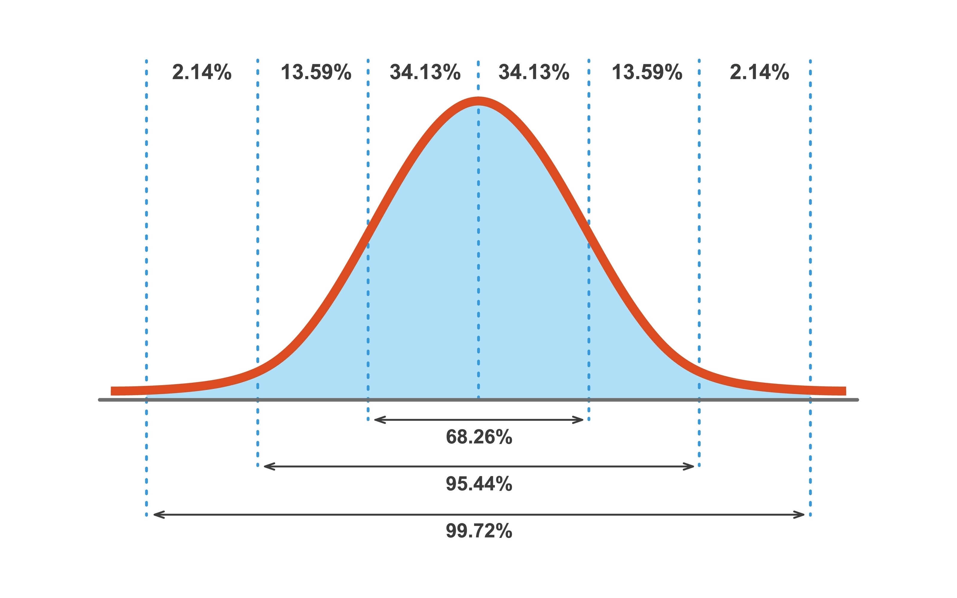Visualizing the “Safety Net”: The shaded area represents the range where we are 95% confident the true mean lies.

---

🐍 Python in Practice: Calculating & Plotting

Theory is great, but let’s see it in action. We will calculate the interval and then visualize it using matplotlib.

import numpy as np
import scipy.stats as stats
import matplotlib.pyplot as plt

# 1. Create a sample dataset (simulating 60 parents)
np.random.seed(42)
data = np.random.normal(loc=2.6, scale=0.8, size=60)

# 2. Calculate Stats
mean_val = np.mean(data)
std_error = stats.sem(data)
confidence_level = 0.95
degrees_freedom = len(data) - 1

# 3. Calculate Interval (T-Distribution)
ci_low, ci_high = stats.t.interval(confidence_level, degrees_freedom, mean_val, std_error)

print(f"Mean: {mean_val:.2f}")
print(f"95% CI: ({ci_low:.2f}, {ci_high:.2f})")

# 4. Visualizing the "Safety Net"
plt.figure(figsize=(10, 6))
# Plot the distribution curve
x = np.linspace(mean_val - 4*std_error, mean_val + 4*std_error, 100)
y = stats.t.pdf(x, degrees_freedom, mean_val, std_error)
plt.plot(x, y, label='Sampling Distribution', color='blue')

# Shade the Confidence Interval (The Safety Net)
x_ci = np.linspace(ci_low, ci_high, 100)
y_ci = stats.t.pdf(x_ci, degrees_freedom, mean_val, std_error)
plt.fill_between(x_ci, y_ci, color='skyblue', alpha=0.4, label='95% Confidence Interval')

plt.axvline(mean_val, color='red', linestyle='--', label=f'Point Estimate ({mean_val:.2f})')
plt.title("Visualizing the 95% Confidence Interval")
plt.legend()
plt.show()

---

🥅 Step 2: The Interval Estimate (The “Safety Net”)

To be more accurate, we move to Interval Estimation. Instead of pinning our hopes on a single number, we calculate a range of values.

This is done by taking your Point Estimate ($\bar{x}$) and adding a “buffer zone” known as the Margin of Error.

📐 How is the Margin of Error calculated?

The formula for a Confidence Interval is:

$$\text{Interval} = \bar{x} \pm \left( Z \times \frac{s}{\sqrt{n}} \right)$$

• \(\bar{x}\): Sample Mean (2.6 hours)
• \(Z\): Confidence Value (usually 1.96 for 95%)
• \(\frac{s}{\sqrt{n}}\): Standard Error (based on variance and sample size)

The part in the brackets is your Margin of Error.

In our example, let’s say the math gives us a margin of ± 0.3 hours.

The Result: “The true average sleep loss is between 2.3 and 2.9 hours.”

✅ This is much safer. We aren’t saying the answer is exactly 2.6; we are saying it’s somewhere in that neighborhood.

---

🛡️ Step 3: Adding Confidence

Intervals come with a Confidence Level—usually set at 95%.

This means: “If we repeated this study 100 times with different samples, 95 of the calculated intervals would contain the true population average.”

So, our final robust conclusion is:

“We are 95% confident that new parents in Amsterdam lose between 2.3 and 2.9 hours of sleep.”

---

✅ Best Practices for Estimation

• Sample Randomly: Your sample must represent the population (e.g., don't just ask parents who drink coffee late at night).
• Use Intervals for Reporting: Whenever possible, report a range (Confidence Interval) rather than just a single number (Point Estimate).
• Check Sample Size: Larger samples generally lead to narrower, more precise intervals.
• State Your Confidence: Always specify if you are 90%, 95%, or 99% confident in your results.

---

⚠ Common Pitfalls to Avoid

• Confusing Sample with Population: Remember, $\bar{x}$ (sample mean) is just an estimate of $\mu$ (population mean).
• Ignoring Uncertainty: Presenting a Point Estimate as an absolute fact can be misleading.
• Bias: If your sample isn't random (e.g., you only asked unhappy parents), your estimate will be wrong regardless of the math.
• Misinterpreting Confidence: 95% confidence doesn't mean there is a 95% chance the parameter is in the interval; it describes the reliability of your method.

---

🧠 Level Up: The Two Main Types of Inferential Statistics

Inferential statistics generally falls into two buckets:

• 📊 Estimation: What we discussed today. Guessing a parameter (like an average) using Point or Interval estimates.
• 🧪 Hypothesis Testing: Testing a specific theory. For example, claiming "Parents lose more than 3 hours of sleep" and using data to prove or disprove it.

Both rely on the same underlying math distributions (like the Normal Distribution or T-Distribution).

---

📌 Try It Yourself: Inferential Statistics & Estimation

Q1: What is the main goal of Inferential Statistics?

💡 Show Answer

To take data from a small sample and make conclusions or predictions about a larger population.

Q2: What is the difference between a Point Estimate and an Interval Estimate?

💡 Show Answer

A Point Estimate uses a single value (like the sample mean) to guess the population parameter. An Interval Estimate provides a range of values (like a confidence interval) where the true parameter likely falls.

Q3: Why is Interval Estimation generally considered "safer" than Point Estimation?

💡 Show Answer

Because it accounts for uncertainty. It acknowledges that the sample might not perfectly match the population and gives a "buffer zone" (margin of error) to increase the chance of capturing the true value.

Q4: If you calculate a 95% Confidence Interval, what does that percentage represent?

💡 Show Answer

It means that if you repeated the study many times with different samples, 95% of the calculated intervals would contain the actual population parameter.

Q5: In the sleep study example, if the sample mean (\( \bar{x} \)) is 2.6 hours, is this the exact population mean (\( \mu \))?

💡 Show Answer

Likely not. The sample mean is just an estimate. The true population mean is unknown but likely falls near 2.6, which is why we calculate an interval around it.

---

Bonus: How does Inferential Statistics apply to Machine Learning?

💡 Show Answer

✅ Generalization: We treat training data as a sample and the real world as the population. We use inferential stats to ensure our model performs well on data it hasn't seen yet, rather than just memorizing the training set.

---

🤖 Why It Matters in Machine Learning

In machine learning, Inferential Statistics is the engine under the hood:

• 🌍 Generalization: Your training data is just a sample. You want your model to work on the “real world” (the population).
• 📉 Model Evaluation: When you say your model has “85% accuracy,” that is a Point Estimate based on your test set. Calculating a Confidence Interval (e.g., 83%-87%) gives you a better idea of real-world performance.
• 🅰️ A/B Testing: Deciding which version of a website performs better relies entirely on comparing samples to infer population behavior.

Understanding estimation helps you stop treating your training data as the “whole truth” and start treating it as a “clue” to the bigger picture.

---

---

🐍 Python in Practice: Calculating Confidence Intervals

Theory is great, but how do we calculate this in Python? We can use the scipy library to generate a confidence interval for our sleep data.

import numpy as np
import scipy.stats as stats

# 1. Create a sample dataset (e.g., sleep loss in hours)
data = [2.1, 2.4, 2.6, 2.8, 2.3, 2.9, 2.5, 2.7, 2.2, 2.6]

# 2. Calculate the Mean (Point Estimate)
mean_val = np.mean(data)

# 3. Calculate the Confidence Interval (95%)
# We use the t-distribution because our sample size is small (<30)
confidence_level = 0.95
degrees_freedom = len(data) - 1
sample_standard_error = stats.sem(data)

interval = stats.t.interval(confidence_level, degrees_freedom, mean_val, sample_standard_error)

print(f"Point Estimate: {mean_val}")
print(f"95% Confidence Interval: {interval}")

Point Estimate: 2.51
95% Confidence Interval: (2.33, 2.69)

---

💡 Pro Tip: When to use Z-Score vs. T-Score?

• Use T-Score (`stats.t.interval`): When your sample size is small ($n < 30$) or—crucially—when you don't know the true population standard deviation (which is almost always the case in real life). The T-distribution is slightly wider ("fatter tails") to account for the extra uncertainty.
• Use Z-Score (`stats.norm.interval`): When you have a massive sample size ($n > 30$) or you somehow know the population's exact standard deviation.

In our Python example, even though we simulated data, we used T because it's the safer, standard approach for estimation.

---

✅ Summary

Method	Definition	Pros/Cons	Example
Point Estimate	A single value guess	Simple, but high error risk	“Mean is 2.6 hours”
Interval Estimate	A range of values	Complex, but captures uncertainty	“Mean is 2.3 - 2.9 hours”

🧠 Takeaway: Always prefer the “Safety Net” (Intervals) over the “Bullseye” (Points) when making important decisions.

---

💬 Got a question or suggestion?

Leave a comment below — I’d love to hear your thoughts on how you use estimation in your data projects!

---

🔜 Up Next

Next, we’ll dive into the second pillar of Inferential Statistics: Hypothesis Testing — how to mathematically prove (or disprove) a theory about your data.