What Are Random Variables and How Do We Visualize Their Distributions?
Learn how to understand and visualize random variables using PMF, PDF, and CDF. Covers discrete vs continuous distributions with real examples and intuitive plots.
What’s the difference between a PMF, PDF, and CDF — and how do they relate to random variables? In this post, we’ll break down the key types of random variables (discrete vs continuous), show you how to visualize them, and explain how these concepts power real-world applications in statistics and machine learning. —
📚 This post is part of the "Intro to Statistics" series
🔙 Previously: Understanding Independence and Bayes’ Rule
🎲 What Is a Random Variable?
A random variable is a numerical outcome of a random phenomenon.
It can take different values depending on the situation — like the result of a die roll, the temperature in your city, or a person’s height.
🧱 Types of Random Variables
| Type | Description | Examples |
|---|---|---|
| Discrete | Takes a countable number of values | # of calls/day, die roll result |
| Continuous | Takes any value within an interval (infinite possibilities) | Height, temperature, weight |
📊 How Do We Work With Random Variables?
We use probability distributions to describe how likely each outcome is.
A probability distribution can be expressed as:
- A table
- A graph
- An equation
Depending on the variable type, we use:
| Type | Distribution Function |
|---|---|
| Discrete | Probability Mass Function (PMF) |
| Continuous | Probability Density Function (PDF) |
🔍 Visual: PMF (Discrete Distribution)
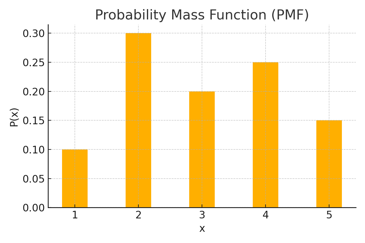
Each bar shows the probability of an exact outcome.
🔍 Visual: PDF (Continuous Distribution)
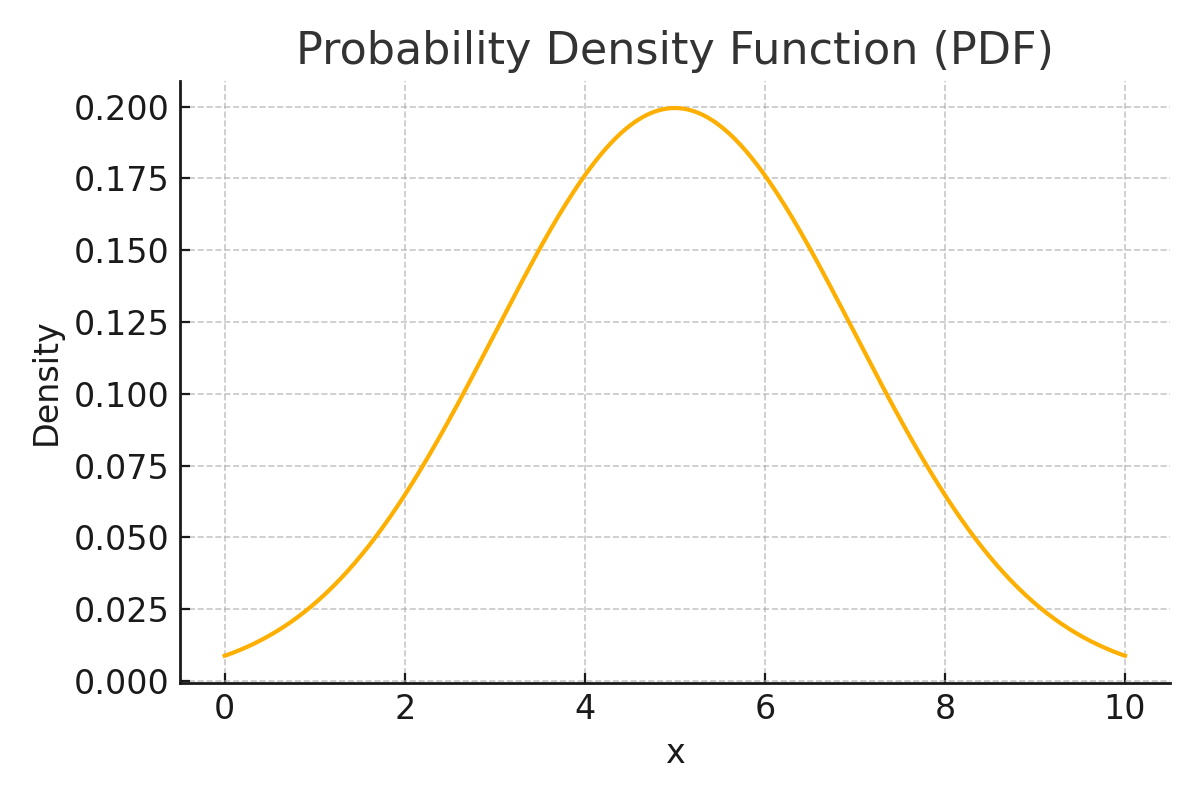
The area under the curve (not the height) represents probability.
You can’t directly say \( P(X = 5) \); it’s always \( P(a \le X \le b) \).
⚖️ Why Are Discrete Probabilities Simpler?
With discrete random variables, calculating probabilities is straightforward — you can just add up the values:
\( P(X = 2 \text{ or } X = 3) = P(X = 2) + P(X = 3) \)
In contrast, with continuous variables, you need to integrate the area under the curve — which often requires formulas or software.
📈 Cumulative Distribution Function (CDF)
The Cumulative Distribution Function answers:
What is the probability that \( X \) is less than or equal to some value?
We can compute CDFs for both discrete and continuous variables.
🧪 Example: CDF (Discrete)
| x | P(X = x) | P(X ≤ x) |
|---|---|---|
| 1 | 0.1 | 0.1 |
| 2 | 0.3 | 0.4 |
| 3 | 0.2 | 0.6 |
| 4 | 0.25 | 0.85 |
| 5 | 0.15 | 1.0 |
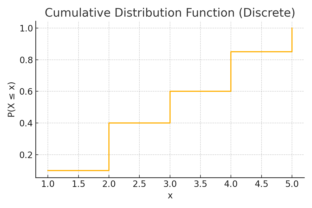
Each step adds the probability from the previous value.
📊 Example: CDF (Continuous)
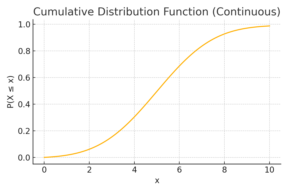
This curve shows P(X ≤ x) for every point — and it always increases.
📉 Distribution vs Cumulative: Visual Comparison
| View | What It Shows |
|---|---|
| PDF / PMF | Probability of individual values (or areas) |
| CDF | Cumulative probability up to a certain point |
🎨 Visual Comparison
PDF → Use the area under curve to find probability
CDF → Read probability directly from the graph
📌 Key Properties of CDF
- Always increases (never decreases)
- Final value = 1
- You can find \( x \) for a given probability — or the other way around
🎯 What Is a Quantile?
A quantile tells us the value at a certain cumulative probability.
- The median is the 0.5 quantile → 50% of values lie below
- The 0.9 quantile means 90% of values are below that point
🔍 Visual Example
If the 90th percentile is 8.1, then \( P(X \le 8.1) = 0.90 \)
🤖 Why It Matters for Machine Learning
In machine learning, understanding random variables and their distributions is essential for:
- Modeling prediction uncertainty (e.g., probabilistic classifiers)
- Evaluating models (e.g., CDFs in ROC analysis)
- Data generation (e.g., sampling from PDFs or PMFs)
- Feature engineering (quantile normalization, log transformations)
Mastering these basics helps you build better models with interpretable results.
🧠 Level Up: Why CDFs Are Powerful
✅ Best Practices
- Use CDFs when comparing distributions or setting thresholds.
- Choose PMF for count data and PDF for continuous measurements.
- Use visualizations to detect skewness or outliers in distributions.
- Verify the total probability sums to 1 in your PMF/PDF.
⚠️ Common Pitfalls
- ❌ Misinterpreting PDF height as probability — area matters.
- ❌ Forgetting that continuous variables can't have P(X = a) > 0.
- ❌ Confusing quantiles with raw values or assuming symmetry.
- ❌ Using PMF formulas on continuous data or vice versa.
📌 Try It Yourself
Q: What’s the key difference between discrete and continuous random variables?
💡 Show Answer
✅ Discrete variables take countable values (like 0, 1, 2...), while Continuous variables can take any value within a range (like height or time).
Q: What is the distribution function for discrete random variables called?
💡 Show Answer
✅ It’s called the Probability Mass Function (PMF) — it gives the probability of each possible value.
Q: Why is it easier to calculate probabilities with discrete variables than continuous ones?
💡 Show Answer
✅ Because you can just sum the individual probabilities. Continuous variables need integration over intervals.
Q: What does the Cumulative Distribution Function (CDF) tell us?
💡 Show Answer
✅ It shows the cumulative probability that a variable is less than or equal to a certain value.
Q: What is a quantile in statistics?
💡 Show Answer
✅ A quantile is a value below which a given percentage of data falls.
For example, the median is the 0.5 quantile.
Bonus: What’s the probability that a continuous variable takes an exact value?
💡 Show Answer
✅ Zero.
We calculate probability over intervals — single values have zero probability in continuous distributions.
✅ Summary
| Concept | Description |
|---|---|
| Random Variable | Represents numeric outcome of a random event |
| Discrete | Countable outcomes (use PMF) |
| Continuous | Infinite outcomes (use PDF) |
| PMF / PDF | Describe probability distribution |
| CDF | Accumulated probability up to x |
| Quantile | Inverse of CDF — get x for a given probability |
🔜 Up Next
In the next post, we’ll explore summary statistics like:
- Mean
- Variance
- Standard deviation
- Expected value
These help us describe how a probability distribution behaves.
Stay tuned!
📺 Explore the Channel

🎥 Hoda Osama AI
Learn statistics and machine learning concepts step by step with visuals and real examples.
💬 Got a Question?
Leave a comment or open an issue on GitHub — I love connecting with other learners and builders. 🔁