⚙️ Optimization in Machine Learning: From Gradient Descent to Newton’s Method

---

⚙️ What Is Optimization in ML?

Optimization is the core process that drives learning in machine learning models.
It’s how we find the best parameters — like weights in a neural network — that reduce error as much as possible.

Imagine you’re hiking through a mountainous landscape: the goal is to reach the lowest valley.
This landscape represents the loss surface, and optimization algorithms guide your steps to find that minimum.

---

---

📚 This post is part of the "Intro to Calculus" series

🔙 Previously: What is the Hessian? Understanding Curvature and Optimization in Machine Learning

---

---

🎯 Loss Functions

A loss function measures how far off a model’s predictions are from actual labels.

Examples:

• Mean Squared Error: \( L = \frac{1}{n}\sum (y_i - \hat{y}_i)^2 \)
• Cross-Entropy for classification

We want to minimize the loss by adjusting parameters.

---

🔽 Gradient Descent (First-Order)

Gradient descent uses the gradient (first derivative) to take steps in the direction of steepest decrease.

Update rule: \[ \theta_{\text{next}} = \theta - \eta \cdot \nabla L(\theta) \]

• \( \eta \): learning rate (step size)
• \( \nabla L(\theta) \): gradient of the loss function

Too large \( \eta \) → overshooting; too small → slow convergence.

---

📉 Python: Gradient Descent Demo

import numpy as np
import matplotlib.pyplot as plt

# Loss function and derivative
f = lambda x: x**2
df = lambda x: 2*x

x_vals = [2.0]  # starting point
lr = 0.1

for _ in range(10):
    x_new = x_vals[-1] - lr * df(x_vals[-1])
    x_vals.append(x_new)

# Plot
x = np.linspace(-2, 2, 100)
y = f(x)
plt.plot(x, y)
plt.scatter(x_vals, [f(x) for x in x_vals], color='red')
plt.title("Gradient Descent on f(x) = x²")
plt.xlabel("x")
plt.ylabel("f(x)")
plt.show()

---

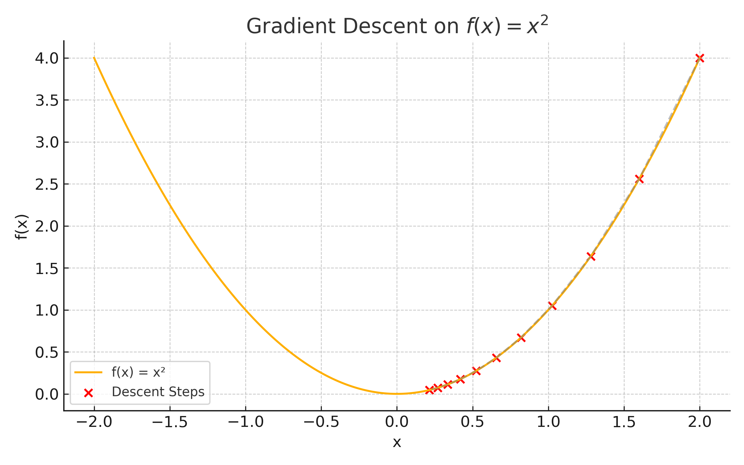
📊 Visual: Gradient Descent Steps on a Curve

This plot shows how gradient descent iteratively steps toward the minimum on ( f(x) = x^2 ):

---

🧠 Newton’s Method (Second-Order)

Newton’s method uses the Hessian to adjust step size based on curvature:

\[ \theta_{\text{next}} = \theta - H^{-1} \nabla L(\theta) \]

Where:

• \( H \): Hessian matrix (second derivatives)
• More accurate near optima, but requires expensive matrix inversion.

---

🧪 Python: Newton’s Method Symbolic (2D)

import sympy as sp

x, y = sp.symbols('x y')
f = x**2 + y**2

# Gradient
grad = sp.Matrix([sp.diff(f, var) for var in (x, y)])
# Hessian
H = sp.hessian(f, (x, y))

# Newton step
theta = sp.Matrix([x, y])
theta_next = theta - H.inv() * grad
sp.simplify(theta_next)

---

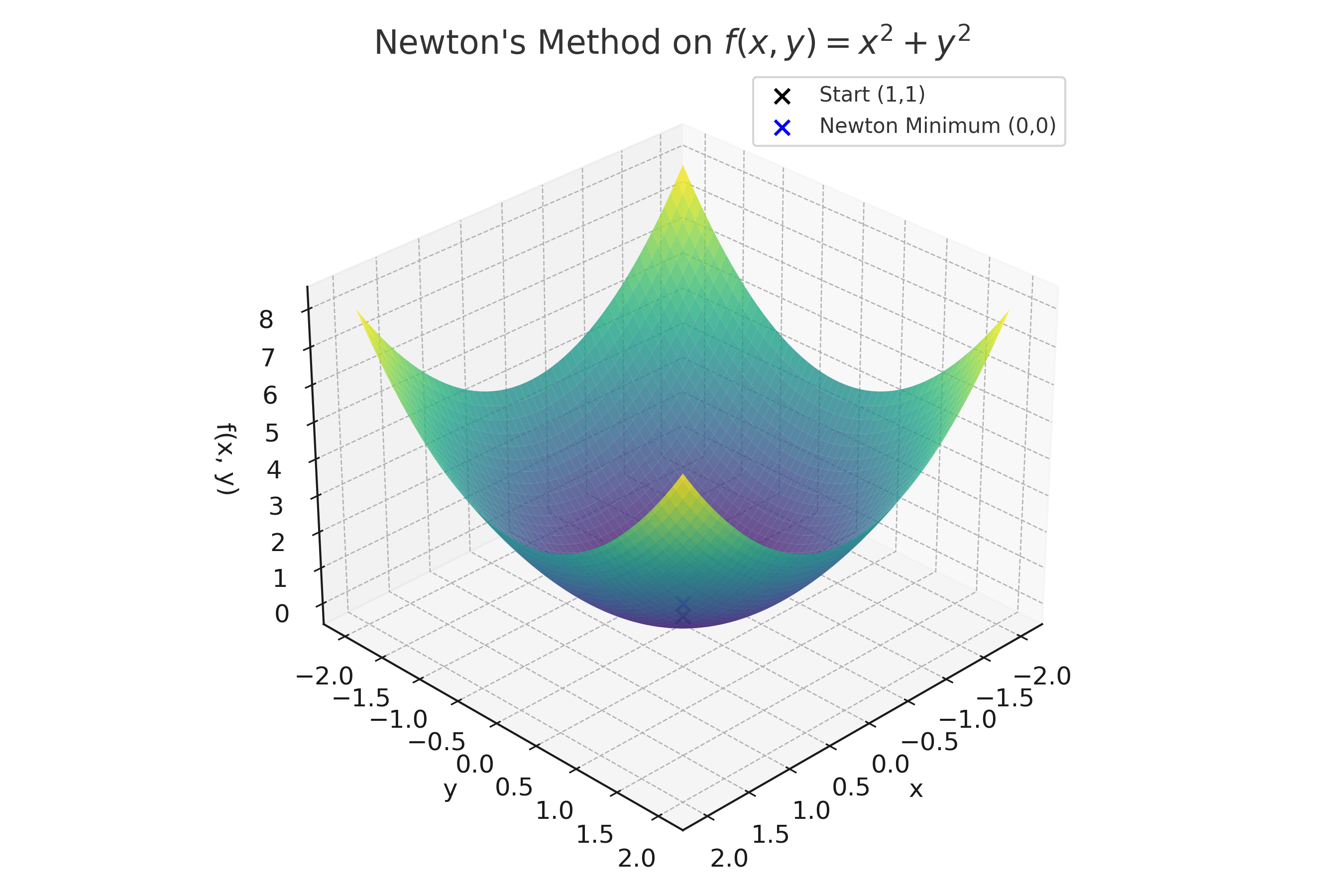
🖼️ Visual: Newton’s Method and Curvature

This 3D surface shows how Newton’s Method uses curvature to jump directly to the bottom:

• Red arrow = gradient direction
• Blue point = Newton’s update lands at the minimum

---

⚖️ Comparing First- and Second-Order Methods

Method	Uses	Pros	Cons
Gradient Descent	First derivative	Simple, scalable	Slower convergence
Newton’s Method	Second derivative	Faster near minimum	Expensive (Hessian inverse)

---

🤖 Relevance to Machine Learning

Optimization is the engine behind how machine learning models learn. Whether it’s a simple linear model or a deep neural network, optimization determines how the model improves its predictions over time.

• Model Training: Algorithms like gradient descent adjust weights to minimize loss functions — it's how models learn from data.
• Neural Networks: Every training step in deep learning is an optimization update, typically using stochastic gradient descent or its variants.
• Convex vs. Non-Convex Loss: Optimization challenges differ depending on whether the loss surface is smooth and convex (easy) or full of local minima/saddles (hard).
• Learning Rate Tuning: Choosing the right learning rate is essential — too small and the model learns slowly, too large and it may diverge.
• Advanced Optimizers: Algorithms like Adam, RMSProp, and L-BFGS use momentum, adaptive learning rates, or curvature approximations to improve training.
• Batch Training: Optimization behaves differently when using mini-batches, full batches, or stochastic updates.
• Loss Surface Geometry: Understanding optimization gives insight into why some models get stuck in saddle points, overshoot, or fail to converge.

---

🧠 Level Up

• 🧭 Optimization = Learning: Every ML model “learns” by minimizing a loss function — optimization is the engine behind it.
• 🚀 Gradient Descent: First-order methods are simple and scale well, making them the default in most neural networks.
• 🔁 Learning Rate Tuning: Adjusting the learning rate can mean the difference between convergence and failure — even for the same algorithm.
• 🔺 Newton’s Method: Second-order updates use curvature to move faster near minima — especially in low-dimensional or convex problems.
• 🧠 Adaptive Methods: Optimizers like Adam and RMSProp approximate curvature and adjust step sizes automatically per parameter.

---

✅ Best Practices

• 🧠 Understand the loss surface: Visualizing or analyzing loss curvature helps choose the right optimizer and learning rate.
• 🔢 Start with simple functions: Practice gradient descent and Newton’s method on 1D and 2D functions to build intuition.
• 📉 Tune the learning rate: Test multiple values — even the best optimizer fails with a poor step size.
• 🔁 Compare first and second-order updates: Understand when Newton’s method outperforms basic gradient descent (e.g., near optima).
• ⚙️ Use auto-diff tools: Frameworks like TensorFlow and PyTorch compute gradients and Hessians efficiently and correctly.

---

⚠️ Common Pitfalls

• ❌ Choosing a bad learning rate: Too large and you overshoot; too small and training stalls.
• ❌ Ignoring convergence behavior: Watch for oscillation, divergence, or vanishing updates.
• ❌ Over-relying on Newton’s method: It's powerful, but impractical for high-dimensional models due to Hessian computation.
• ❌ Misinterpreting gradient direction: The gradient shows steepest increase — you must subtract it to minimize loss.
• ❌ Confusing global vs. local minima: Optimization finds local minima — that doesn’t always mean it’s the best possible model.

---

📌 Try It Yourself

📊 Gradient Descent Step: What’s the next value of \( x \) if we start at \( x = 2 \) on \( f(x) = x^2 \) with learning rate 0.1?

🧠 Step-by-step:
- Gradient: \( f'(x) = 2x \), so at \( x = 2 \), \( f'(2) = 4 \)
- Update rule: \( x_{\text{next}} = x - \eta \cdot f'(x) = 2 - 0.1 \cdot 4 = 1.6 \) ✅ Final Answer: \[ x_{\text{next}} = 1.6 \]

---

📊 Newton’s Method Step: On \( f(x) = x^2 \), what is the Newton update from \( x = 2 \)?

🧠 Step-by-step:
- Gradient: \( f'(x) = 2x \), so \( f'(2) = 4 \)
- Hessian (2nd derivative): \( f''(x) = 2 \)
- Newton update: \( x_{\text{next}} = x - \frac{f'(x)}{f''(x)} = 2 - \frac{4}{2} = 0 \) ✅ Final Answer: \[ x_{\text{next}} = 0 \]

---

📊 Compare Steps: Which method moves more aggressively from \( x = 2 \) on \( f(x) = x^2 \)?

🧠 Answer:
- Gradient Descent took \( x \rightarrow 1.6 \)
- Newton’s Method took \( x \rightarrow 0 \)
✅ Newton's Method is more aggressive and goes straight to the minimum in this case.

---

🔁 Summary: What You Learned

🧠 Concept	📌 Description
Loss Function	Measures model error — optimization tries to minimize it
Gradient Descent	First-order method that uses slope to step toward minima
Learning Rate	Controls step size — critical for convergence
Newton’s Method	Uses both gradient and Hessian for curvature-aware optimization
Hessian Matrix	Matrix of second derivatives — shows local curvature
Convex vs Non-Convex	Optimization behavior changes based on loss surface shape
Optimizer Behavior	Different optimizers converge at different speeds and directions
Python Tools	Libraries like NumPy and SymPy can simulate and visualize optimization steps

---

💬 Got a question or suggestion?

Leave a comment below — I’d love to hear your thoughts or help if something was unclear.