Measuring the Center: Mean, Median, and Mode Explained

Before analyzing how your data spreads, it’s essential to understand how to measure its center. This post introduces the three most important measures of central tendency — mean, median, and mode — with examples, Python code, and practical advice for data science and machine learning.

---

📚 This post is part of the "Intro to Statistics" series

🔙 Previously: How to Build Frequency Tables in Python

🔜 Next: Measures of Dispersion: Range, IQR, and Box Plot

---

🎯 What is Central Tendency?

Central tendency describes the “middle” or typical value in a dataset. The three main measures are:

• Mode
• Median
• Mean

Each one tells us something slightly different.

---

🧮 Mode

• The most frequent value in a dataset
• Works with any type of variable
• Especially useful for nominal (categorical) data

💡 Example:
If most students choose “Math” as their favorite subject, then:

Mode = “Math”

🛑 You can’t calculate a mean or median for categories like “Math” or “History” — but you can find the mode.

Tip:
A dataset can have more than one mode (bi-modal or multi-modal), or no mode at all if all values occur with the same frequency.

from scipy import stats
data = [80, 90, 85, 90, 95, 90, 92]
mode = stats.mode(data, keepdims=True)
print("Mode:", mode.mode[0])

---

🧭 Median

• The middle value when data is sorted
• Best used when data is skewed or has outliers
• Only works with ordinal, interval, or ratio variables

💡 Example:
For ages: [16, 17, 18, 40, 90]

Median = 18

✅ Median is not affected by extreme values — that’s why it’s preferred when there are outliers.

import numpy as np
data = [16, 17, 18, 40, 90]
median = np.median(data)
print("Median:", median)

---

➕ Mean

• The arithmetic average
• Add up all values, divide by the count

\[ \text{Mean} = \bar{x} = \frac{1}{n} \sum_{i=1}^{n} x_i \]

Where:

• ( x_i ) = each observation
• ( n ) = total number of observations

💡 Example:
Scores = [80, 85, 90]
\[ \bar{x} = \frac{80 + 85 + 90}{3} = \frac{255}{3} = 85 \]

🛑 Not ideal when there are outliers — they can distort the average.

import numpy as np
scores = [80, 85, 90]
mean = np.mean(scores)
print("Mean:", mean)

---

Note:
There are other means, such as the geometric mean (useful for multiplicative data or log scales) and harmonic mean (used in F1-score for classification). For most ML tasks, the arithmetic mean, median, and mode are most common.

---

🖼️ Visual Comparison

Here’s a quick visual to help you compare the three measures:

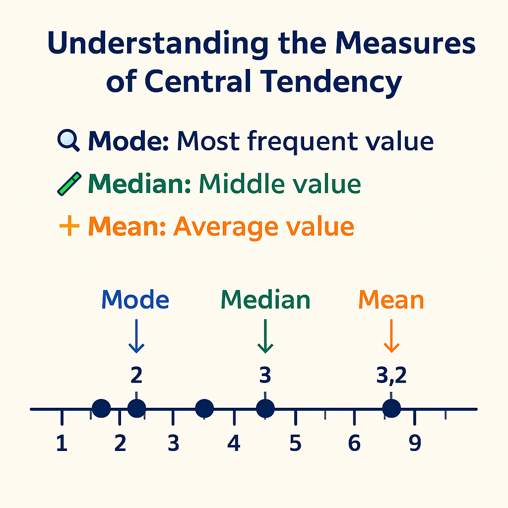
• Mode = Most frequent
• Median = Middle value
• Mean = Balances all data values

---

📌 Choosing the Right Measure

Measurement Level	Mode	Median	Mean
Nominal	✅	❌	❌
Ordinal	✅	✅	❌
Interval/Ratio	✅	✅	✅

⚠️ Outliers = values that are much higher or lower than the rest
👉 When outliers exist, median is often more reliable than mean.

🤖 Why Central Tendency Matters in Machine Learning

• Data Cleaning: Mean, median, or mode are often used to fill missing values in features.
• Feature Engineering: Central tendency measures summarize features for model input or reporting.
• Outlier Detection: Comparing mean and median helps spot skewed data or outliers that may affect model performance.
• Class Imbalance: The mode is used to check the most common class in classification problems.

• Distribution Comparison: Comparing mean/median before and after scaling or transformation helps assess preprocessing effects.

  In short, understanding mean, median, and mode is essential for preparing, analyzing, and interpreting data in any machine learning project.

---

👉 Real-World ML Example Table

Scenario	Best Measure	Why
Filling missing values in income data	Median	Robust to outliers
Most common class in classification	Mode	Identifies class imbalance
Average pixel value in images	Mean	Used in normalization
Skewed housing prices	Median	Not distorted by high outliers

---

📌 Try It Yourself

Q: In a neighborhood of 9 houses, 8 are priced between $300,000 and $350,000, but 1 is a mansion worth $3.5 million.

Which measure of central tendency would best describe the typical house price in this neighborhood?

💡 Show Answer

✅ Median — because it’s resistant to extreme values like the mansion.

The mean would be skewed upward by the $3.5M value, but the median stays closer to what most houses are actually worth.

---

Bonus: What is the only measure of central tendency suitable for categorical (non-numeric) data?

💡 Show Answer

✅ Mode — it identifies the most frequently occurring category.

For example, if most people in a survey choose “Cat” as their favorite pet, then the mode is “Cat”.

---

⚠️ Common Pitfalls

• Using mean with skewed or outlier-heavy data (use median instead).
• Using mean or median for categorical data (use mode).
• Forgetting that multi-modal data can have more than one mode.
• Not sorting data before finding the median.
• Assuming the mean always represents the “typical” value, even when the data is skewed.

---

🧠 Level Up: When and Why to Choose Mode, Median, or Mean

Each measure of center has its strengths depending on the data and the question:

• 📌 Mode is great for identifying the most common category or value — useful in marketing, survey analysis, and categorical data.
• 📌 Median provides a robust center when your data has outliers or is skewed — like income or house prices.
• 📌 Mean is ideal when data is symmetrically distributed and you want to use all values — common in scientific measurements and many ML algorithms.

Knowing when to use each makes your analysis more accurate and meaningful.

---

🔁 Summary

Measure	Best For	Sensitive to Outliers?
Mode	Nominal, any variable	❌ No
Median	Skewed/Ordinal data	❌ No
Mean	Symmetrical data only	✅ Yes

---

💬 Got a question or suggestion?
Let me know in the comments below — whether it’s about understanding central tendency or applying it to your ML dataset.

---

✅ Up Next

In the next post, we’ll talk about how spread out your data is.
That’s called Measures of Dispersion — including Range, Interquartile Range, and the Box Plot.

Stay curious!