🔗 Chain Rule, Implicit Differentiation, and Partial Derivatives (Calculus for ML)

Before diving into neural networks or complex optimization, it’s critical to master three powerful tools in calculus: the Chain Rule, Implicit Differentiation, and Partial Derivatives.

In this post, you’ll learn:

• How to apply the chain rule to composite functions
• How implicit differentiation builds on the chain rule
• How to differentiate multivariable functions with respect to one variable (partial differentiation)

---

📚 This post is part of the "Intro to Calculus" series

🔙 Previously: Understanding Gradients and Partial Derivatives (Multivariable Calculus for Machine Learning)

🔜 Next: Understanding the Jacobian – A Beginner’s Guide with 2D & 3D Examples

---

🔗 What is the Chain Rule?

The chain rule allows us to differentiate composite functions, i.e., functions inside other functions.

Let’s say:

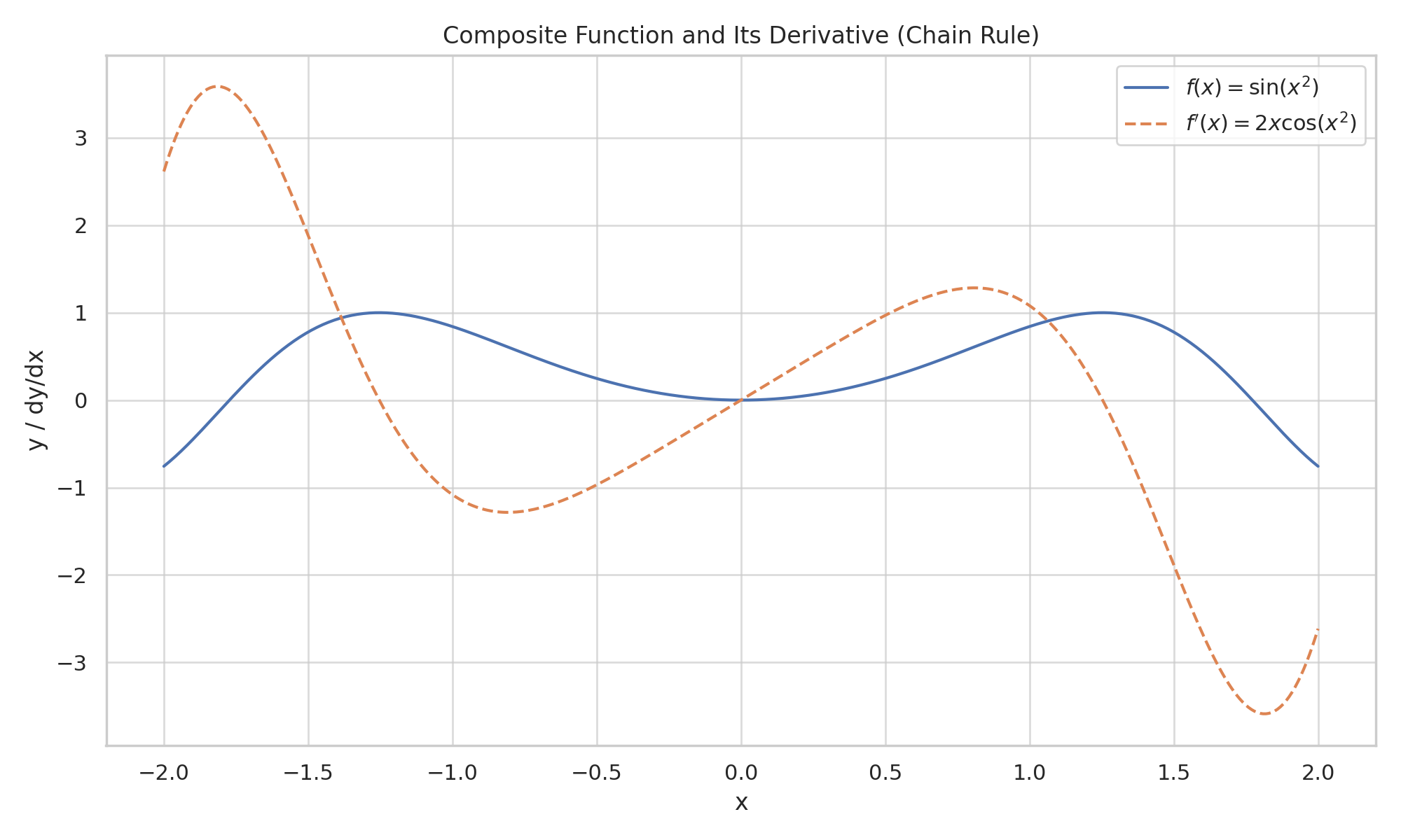
\[ f(x) = h(p(x)) = \sin(x^2) \]

We treat the outer function \( h(u) = \sin(u) \), and the inner \( p(x) = x^2 \).

Using the chain rule:

\[ f’(x) = h’(p(x)) \cdot p’(x) = \cos(x^2) \cdot 2x \]

✅ So, the derivative of \( \sin(x^2) \) is \( 2x \cdot \cos(x^2) \)

---

🧮 Python: Symbolic Chain Rule

import sympy as sp

x = sp.symbols('x')
f = sp.sin(x**2)
dfdx = sp.diff(f, x)
dfdx = 2*x*cos(x**2)

---

---

🧠 Another Chain Rule Example (Step-by-Step)

Let’s find the derivative of:

\[ f(x) = \ln(3x^2 + 1) \]

This function has a function inside a function, which is exactly when we use the chain rule.

---

🔹 Step 1: Identify the Inner and Outer Functions

We rewrite the function as:

\[ f(x) = h(p(x)) \]

Where:

• The inner function is: \( p(x) = 3x^2 + 1 \)
• The outer function is: \( h(u) = \ln(u) \), with \( u = p(x) \)

---

🔹 Step 2: Differentiate Each Part

• \( h’(u) = \frac{1}{u} \) → this is the derivative of \( \ln(u) \)
• \( p’(x) = \frac{d}{dx}(3x^2 + 1) = 6x \)

Now apply the chain rule:

\[ f’(x) = h’(p(x)) \cdot p’(x) = \frac{1}{3x^2 + 1} \cdot 6x \]

---

✅ Final Answer

\[ f’(x) = \frac{6x}{3x^2 + 1} \]

---

💡 Why This Matters

When differentiating logarithmic, trigonometric, or exponential functions wrapped around polynomials, the chain rule is your go-to tool. You treat the “outside” and “inside” layers separately, then multiply the results.

---

🔁 Implicit Differentiation

Sometimes, functions are not written in the form \( y = f(x) \). Instead, x and y are mixed together in one equation. In that case, we can’t isolate y easily — so we use implicit differentiation.

---

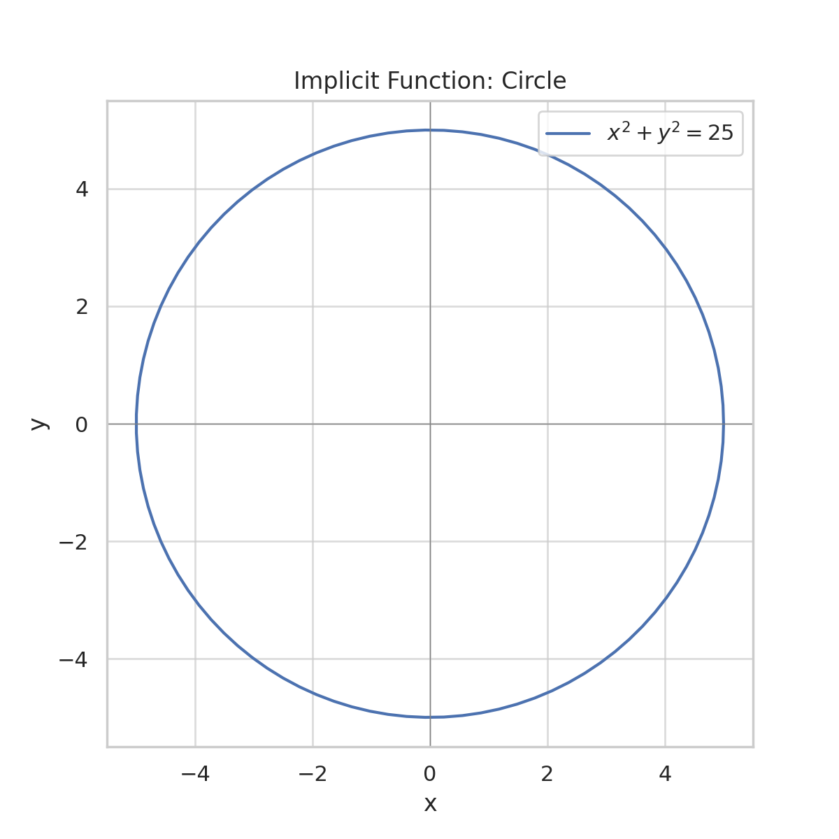
📘 Example: A Circle

Take the equation of a circle:

\[ x^2 + y^2 = 25 \]

This defines a relationship between x and y, but y is not explicitly solved.

---

🧠 Step 1: Differentiate both sides with respect to x

Apply \( \frac{d}{dx} \) to each term:

\[ \frac{d}{dx}(x^2) + \frac{d}{dx}(y^2) = \frac{d}{dx}(25) \]

• \( \frac{d}{dx}(x^2) = 2x \)
• \( \frac{d}{dx}(25) = 0 \) (constants have zero slope)
• \( \frac{d}{dx}(y^2) = 2y \cdot \frac{dy}{dx} \) ← this uses the chain rule, because y is treated as a function of x

So the full result becomes:

\[ 2x + 2y \cdot \frac{dy}{dx} = 0 \]

---

✍️ Step 2: Solve for \( \frac{dy}{dx} \)

Subtract \( 2x \) from both sides:

\[ 2y \cdot \frac{dy}{dx} = -2x \]

Divide both sides by \( 2y \):

\[ \frac{dy}{dx} = \frac{-x}{y} \]

---

💡 Interpretation:

Even though we didn’t solve for y directly, we found the slope of the curve at any point (x, y) on the circle. This is powerful — we differentiated without rearranging!

---

🔗 This method is essential when:

• y appears in powers or multiplied with x
• You have to find \( \frac{dy}{dx} \) but can’t isolate y
• You’re working with geometric shapes, constraint equations, or system-level models in ML

---

---

🔀 Partial Derivatives

When a function depends on more than one variable (e.g., \( f(x, y, z) \)), we can differentiate with respect to one, treating the others as constants.

Let:

\[ f(x, y, z) = \sin(x) \cdot e^{yz^2} \]

🔹 Differentiate with respect to \( x \):

Only \( \sin(x) \) is affected:

\[ \frac{\partial f}{\partial x} = \cos(x) \cdot e^{yz^2} \]

✅ Here, \( y \) and \( z \) are treated as constants.

🔹 Differentiate with respect to ( y ):

\[ \frac{\partial f}{\partial y} = \sin(x) \cdot e^{yz^2} \cdot z^2 \]

Chain rule applied to the exponent!

---

🔹 Differentiate with respect to \( z \):

\[ \frac{\partial f}{\partial z} = \sin(x) \cdot e^{yz^2} \cdot 2yz \]

---

🧮 Python: Symbolic Partial Derivatives

import sympy as sp

x, y, z = sp.symbols('x y z')
f = sp.sin(x) * sp.exp(y * z**2)

df_dx = sp.diff(f, x)
df_dy = sp.diff(f, y)
df_dz = sp.diff(f, z)

df_dx, df_dy, df_dz

Output:

(exp(y*z**2)*cos(x),
 z**2*exp(y*z**2)*sin(x),
 2*y*z*exp(y*z**2)*sin(x))

This confirms our analytical work.

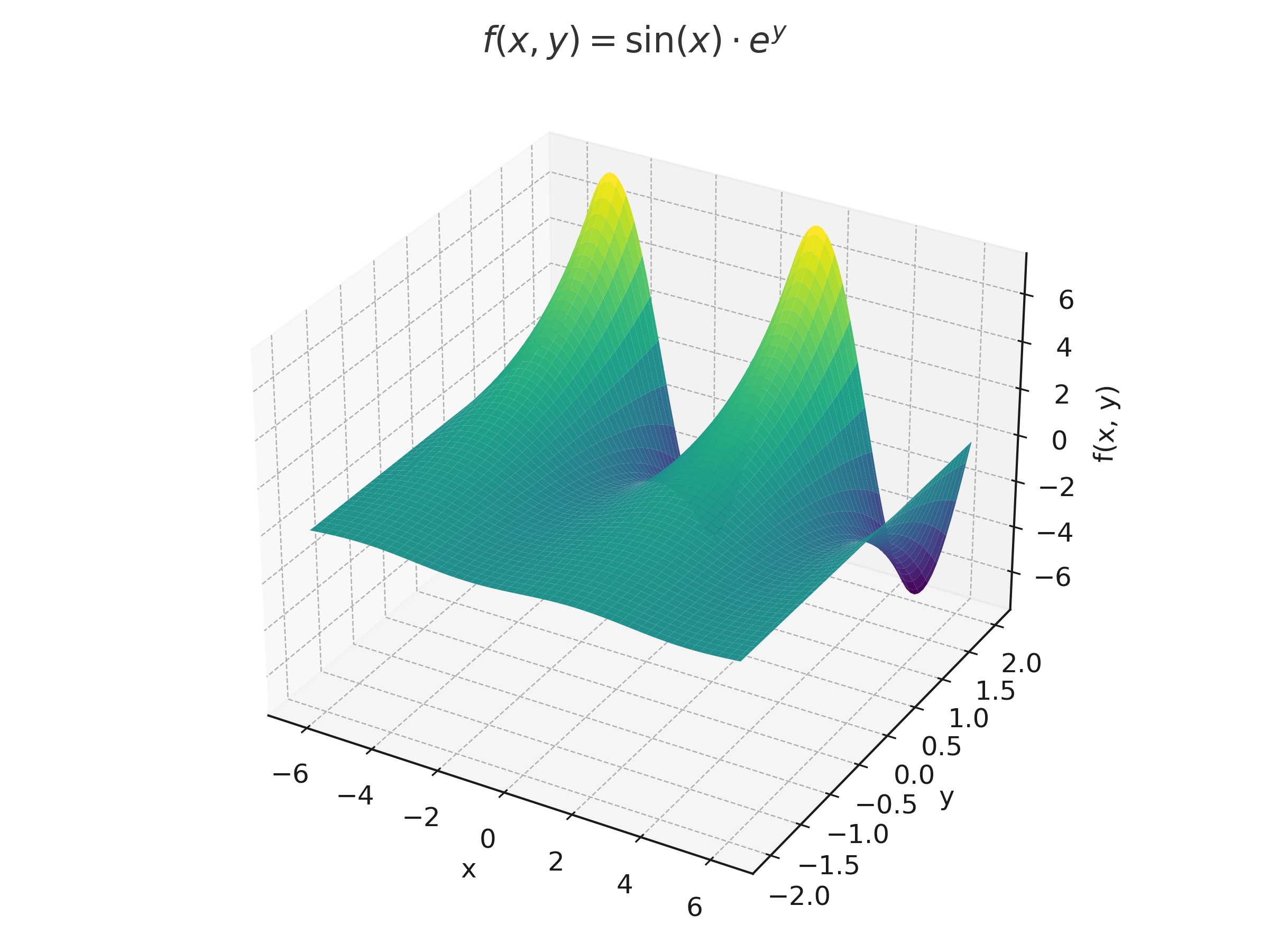
✅ 3. Visualizing f(x, y) = sin(x) · e^y in 3D

`

---

📊 Python: 3D Surface Plot

import numpy as np
import matplotlib.pyplot as plt

X, Y = np.meshgrid(np.linspace(-2*np.pi, 2*np.pi, 100), np.linspace(-2, 2, 100))
Z = np.sin(X) * np.exp(Y)

fig = plt.figure(figsize=(8, 6))
ax = fig.add_subplot(111, projection='3d')
ax.plot_surface(X, Y, Z, cmap='viridis')
ax.set_title(r'$f(x, y) = \sin(x) \cdot e^y$')
ax.set_xlabel('x')
ax.set_ylabel('y')
ax.set_zlabel('f(x, y)')
plt.show()

🤖 Relevance to Machine Learning

Understanding these differentiation tools is essential for anyone working in machine learning:

• 🧮 Chain Rule powers backpropagation in neural networks. Each layer’s gradient is computed by chaining derivatives through the layers — exactly as taught by the chain rule.
• ⚙️ Partial Derivatives form the backbone of gradient-based optimization. In functions with multiple variables (e.g., model weights), we compute partials to know how each parameter affects the loss.
• ❓ Implicit Differentiation appears in constrained optimization and in tools like Lagrange Multipliers, often used when variables can’t be expressed directly.
• 📉 These techniques together allow models to learn, update weights, and minimize error during training.

In short: these aren’t just abstract math tricks — they’re the mathematical gears that drive intelligent systems.

---

🚀 Level Up

• 💡 The Chain Rule extends naturally to multiple nested layers — this is the foundation of backpropagation in neural networks.
• 🔁 Implicit Differentiation is especially useful in constraint optimization problems where you can’t isolate a variable.
• 🌐 Partial Derivatives are essential for working with functions of many variables — you'll see them in gradient vectors, Jacobians, and Hessians.
• 📊 In machine learning, partial derivatives guide how each weight is updated during training.
• 🧠 Want to go deeper? Explore the Total Derivative and Directional Derivatives for full control over multivariate calculus.

---

✅ Best Practices

• 🔍 Break down complex expressions into inner and outer layers to apply the chain rule step by step.
• 🧠 Label your inner and outer functions clearly — this reduces mistakes and makes your process transparent.
• 📐 Use implicit differentiation when a function defines x and y together — especially useful for constraint problems.
• 🧮 In partial differentiation, freeze all variables you're not differentiating with respect to — treat them like constants.
• 📊 Simplify before and after differentiating — it helps reduce errors and makes the final expression cleaner.
• 📈 Check your results visually when possible using a graphing tool to confirm slope behavior matches intuition.

---

⚠️ Common Pitfalls

• ❌ Forgetting to multiply by the derivative of the inner function when using the chain rule — the #1 mistake!
• ❌ Applying the power rule directly to composite expressions without unpacking layers first.
• ❌ Misusing implicit differentiation by forgetting to apply the chain rule to y terms.
• ❌ In partial differentiation, accidentally differentiating with respect to more than one variable at once.
• ❌ Confusing constant functions with constant coefficients — constants like 7 are different from terms like 7x.

---

📌 Try It Yourself

Test your understanding with these practice problems. Each one focuses on a key technique: chain rule, implicit differentiation, or partial derivatives.

---

📊 Chain Rule: What is \( \frac{d}{dx} \sin(5x^2) \) ?

This is a composite function: \( \sin(u) \) where \( u = 5x^2 \)
🧠 Step-by-step: - Outer: \( \frac{d}{du} \sin(u) = \cos(u) \) - Inner: \( \frac{d}{dx}(5x^2) = 10x \) ### ✅ Final Answer: \[ \frac{d}{dx} \\sin(5x^2) = \\cos(5x^2) \\cdot 10x \]

---

📊 Implicit Differentiation: Given \( x^2 + xy + y^2 = 7 \), find \( \frac{dy}{dx} \)

Differentiate both sides with respect to \( x \):
🧠 Step-by-step: - \( \frac{d}{dx}(x^2) = 2x \) - \( \frac{d}{dx}(xy) = x \cdot \frac{dy}{dx} + y \) ← product rule! - \( \frac{d}{dx}(y^2) = 2y \cdot \frac{dy}{dx} \) - \( \frac{d}{dx}(7) = 0 \) Putting it together: \[ 2x + x \cdot \frac{dy}{dx} + y + 2y \cdot \frac{dy}{dx} = 0 \] Group \( \frac{dy}{dx} \) terms: \[ (x + 2y)\frac{dy}{dx} = -(2x + y) \] ### ✅ Final Answer: \[ \frac{dy}{dx} = \frac{-(2x + y)}{x + 2y} \]

---

🔁 Summary: What You Learned

🧠 Concept	📌 Description
Chain Rule	Differentiates composite functions by chaining outer and inner derivatives.
Implicit Differentiation	Differentiates equations where y is not isolated, using the chain rule on y terms.
Partial Derivative	Differentiates multivariable functions with respect to one variable at a time.
Backpropagation	Uses chain rule to compute gradients layer by layer in neural networks.
Gradient Vector	A vector of partial derivatives used in optimization and ML training.
Derivative of sin(x²)	\( \frac{d}{dx}\sin(x^2) = 2x \cdot \cos(x^2) \)
∂f/∂x of f(x, y, z)	\( \frac{\partial}{\partial x}(\sin(x)e^{yz^2}) = \cos(x)e^{yz^2} \)

---

💬 Got a question or suggestion?

Leave a comment below — I’d love to hear your thoughts or help if something was unclear.

---

🧭 Next Up

Now that you’ve learned how to compute partial derivatives, you’re ready to tackle the next building block in multivariable calculus: the Jacobian Matrix.

In the next post, we’ll explore:

• What the Jacobian is and how it’s constructed
• Why it’s essential for transformations, coordinate changes, and machine learning gradients
• Step-by-step examples for both scalar and vector-valued functions

Stay curious — you’re one layer closer to mastering the math behind modern ML models.