🔺 What is the Hessian? Understanding Curvature and Optimization in Machine Learning

Posted Jun 22, 2025

By Hoda Osama

9 min read

🔺 What is the Hessian?

In multivariable calculus, the gradient gives us direction — but what about shape?

That’s where the Hessian comes in. It tells us whether we’re in a valley, a ridge, or at a saddle point — and this insight powers many optimization algorithms used in machine learning.

📚 This post is part of the "Intro to Calculus" series

🔙 Previously: Understanding the Jacobian – A Beginner’s Guide with 2D & 3D Examples

🔜 Next: Optimization in Machine Learning: From Gradient Descent to Newton’s Method

🧮 Definition

The Hessian is the square matrix of second-order partial derivatives of a scalar function:

\[ H(f) = \begin{bmatrix} \frac{\partial^2 f}{\partial x^2} & \frac{\partial^2 f}{\partial x \partial y}
\frac{\partial^2 f}{\partial y \partial x} & \frac{\partial^2 f}{\partial y^2} \end{bmatrix} \]

It captures how the gradient changes.
If all second partials are continuous, the Hessian is symmetric.
This symmetry comes from Clairaut’s theorem:
If the second partial derivatives are continuous, then
\( \frac{\partial^2 f}{\partial x \partial y} = \frac{\partial^2 f}{\partial y \partial x} \).

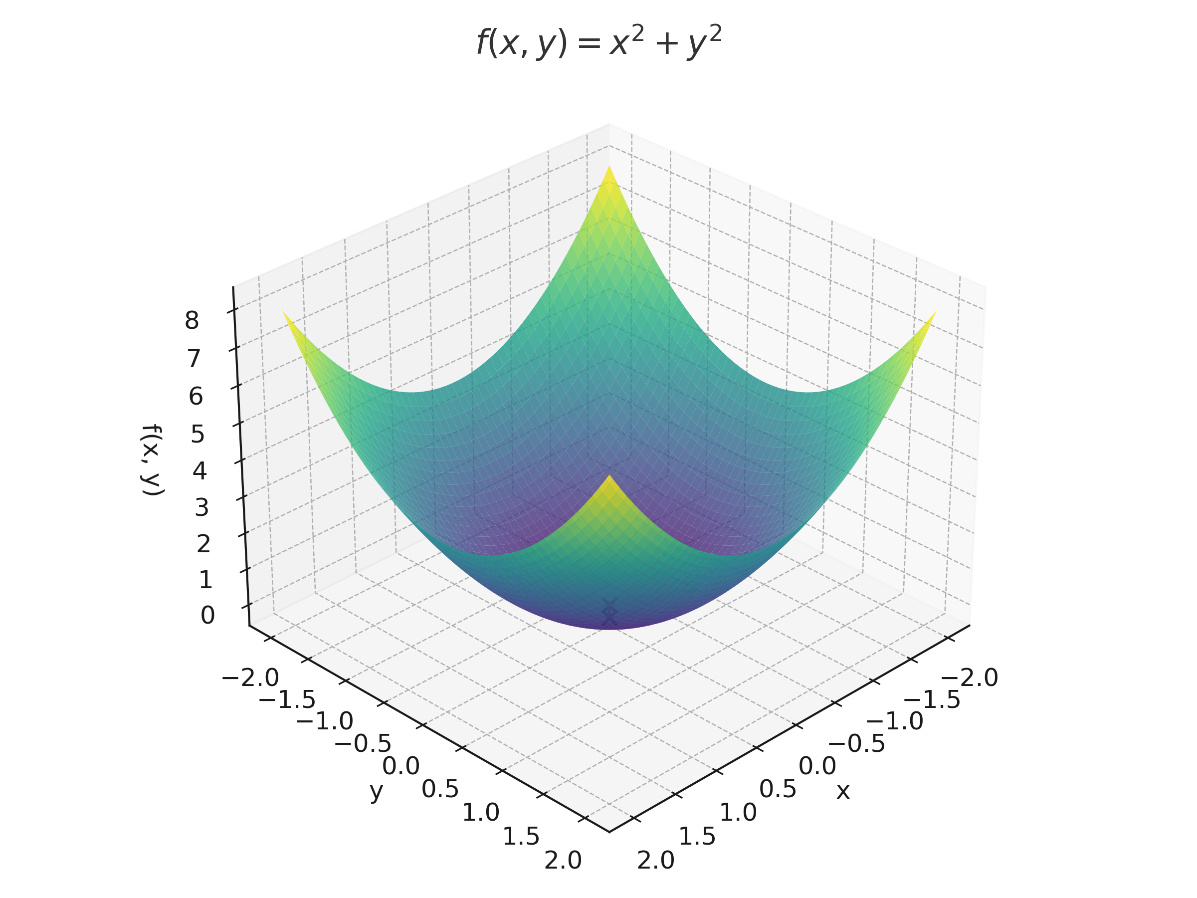
📐 Example: \( f(x, y) = x^2 + y^2 \)

Let’s compute the Hessian:

\[ \frac{\partial^2 f}{\partial x^2} = 2, \quad \frac{\partial^2 f}{\partial y^2} = 2, \quad \frac{\partial^2 f}{\partial x \partial y} = 0 \]

\[ H(f) = \begin{bmatrix} 2 & 0
0 & 2 \end{bmatrix} \]

The matrix is positive definite, so this function is convex everywhere.

🔍 Another Example: \( f(x, y) = x^2 - y^2 \)

\[ \frac{\partial^2 f}{\partial x^2} = 2, \quad \frac{\partial^2 f}{\partial y^2} = -2, \quad \frac{\partial^2 f}{\partial x \partial y} = 0 \]

\[ H(f) = \begin{bmatrix} 2 & 0
0 & -2 \end{bmatrix} \]

The eigenvalues have mixed signs, so this is a saddle point.

🧠 Geometric Meaning

Hessian → curvature matrix
If all eigenvalues > 0: bowl (local minimum)
If all eigenvalues < 0: upside-down bowl (local maximum)
Mixed signs: saddle point

A good function to visualize: \[ f(x, y) = x^2 + y^2 \quad \text{(bowl)}
f(x, y) = x^2 - y^2 \quad \text{(saddle)} \]

🧪 Python: Symbolic Hessian with SymPy

  
import sympy as sp

x, y = sp.symbols('x y')
f = x**2 + y**2

H = sp.hessian(f, (x, y))
H

Output:

  
Matrix([
  [2, 0],
  [0, 2]
])

Now try:

  
f2 = x**2 - y**2
sp.hessian(f2, (x, y))

🖼️ Visualizing Curvature

Use matplotlib or plotly to show:

\( f(x, y) = x^2 + y^2 \): convex bowl
\( f(x, y) = x^2 - y^2 \): saddle

We can also plot contour + gradient + Hessian vector field (advanced, optional).

⚙️ Newton’s Method and Optimization

In optimization, we often want to find the minimum of a function — where the gradient is zero and the curvature is positive.

🔁 First-order update (Gradient Descent)

Gradient descent uses only first derivatives:

\[ \theta_{\text{next}} = \theta - \eta \cdot \nabla f(\theta) \]

Moves in the direction of steepest descent.
Works well, but can be slow if the landscape is curved or poorly scaled.

🧠 Second-order update (Newton’s Method)

Newton’s method adds curvature awareness using the Hessian:

\[ \theta_{\text{next}} = \theta - H^{-1} \nabla f(\theta) \]

Uses the inverse of the Hessian matrix to rescale the gradient.
Adapts step sizes based on how “steep” or “flat” the surface is in different directions.
Can converge faster than gradient descent near minima.

📌 Example: Newton Step in 2D

Suppose:

\[ f(x, y) = x^2 + y^2 \Rightarrow \nabla f = \begin{bmatrix} 2x \\ 2y \end{bmatrix}, \quad H(f) = \begin{bmatrix} 2 & 0 \\ 0 & 2 \end{bmatrix} \]

Then:

\[ \theta_{\text{next}} = \theta - \begin{bmatrix} 2 & 0 \\ 0 & 2 \end{bmatrix}^{-1} \begin{bmatrix} 2x \\ 2y \end{bmatrix} = \theta - \begin{bmatrix} x \\ y \end{bmatrix} \]

This jumps directly to the minimum at \((0, 0)\) in one step!

🧪 Python: Newton’s Method Symbolically

  
import sympy as sp

x, y = sp.symbols('x y')
theta = sp.Matrix([x, y])
f = x**2 + y**2

# Gradient
grad = sp.Matrix([sp.diff(f, var) for var in (x, y)])

# Hessian
H = sp.hessian(f, (x, y))

# Newton step: θ - H⁻¹ ∇f
H_inv = H.inv()
theta_next = theta - H_inv * grad
theta_next

Output:

  
Matrix([
 [0],
 [0]
])

This confirms the Newton step lands exactly at the minimum.

🖼️ Visualizing Newton’s Step

Let’s visualize the function \( f(x, y) = x^2 + y^2 \) and what happens during one Newton update:

We start at point \( (1, 1) \).
The red arrow shows the gradient direction (steepest ascent).
The blue dot shows where Newton’s Method lands — directly at the minimum \( (0, 0) \).

Notice how the Newton step jumps to the bottom in one move — this is the power of incorporating curvature via the Hessian.

🤖 Relevance to Machine Learning

The Hessian matrix plays a powerful role in optimization and training deep learning models:

Second-Order Optimization: Newton’s Method uses the Hessian to adjust step size and direction — it can converge faster than gradient descent, especially near minima.
Curvature Awareness: The Hessian tells us if we're at a valley, ridge, or saddle point. This helps avoid slow progress or divergence in ill-conditioned loss surfaces.
Saddle Point Escape: In high-dimensional neural nets, gradient descent often stalls at saddle points. The Hessian helps identify them and guide escape strategies.
Optimizer Design: Algorithms like L-BFGS and Adam (via approximations) incorporate second-order information to improve training speed and stability.
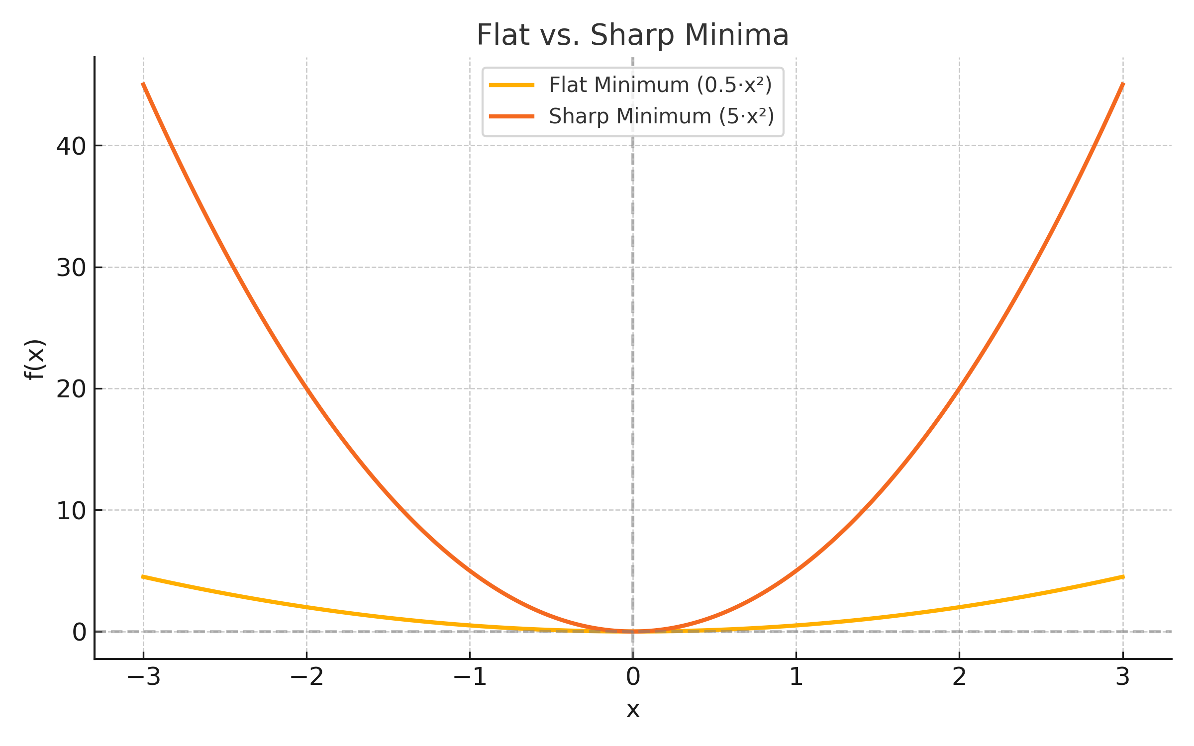
Generalization Diagnostics: The curvature (eigenvalues of the Hessian) is used to study sharp vs. flat minima, which affects how well models generalize to new data.
Loss Landscape Visualization: Hessians enable tools that visualize how “bumpy” or “smooth” a model’s loss function is in parameter space.
In Bayesian optimization, the Hessian of the acquisition function is used to guide sampling.

🎨 Flat vs. Sharp Minima

Understanding curvature helps us reason about model generalization:

Flat minima → gentle curvature, often associated with better generalization.
Sharp minima → steep, narrow curvature, may lead to overfitting.

🧠 Level Up

🔺 Curvature Awareness: The Hessian captures how the gradient changes — it's the second derivative in multivariable calculus.
🚀 Newton’s Method: Instead of just following the gradient, use the Hessian to jump toward minima using second-order updates.
📉 Saddle Point Detection: Mixed-sign eigenvalues in the Hessian help detect saddle points — common in high-dimensional ML models.
🧠 Flat vs. Sharp Minima: The spectrum of the Hessian is used to analyze generalization in deep learning.
🛠️ Advanced Optimizers: Methods like L-BFGS and trust region algorithms approximate or leverage the Hessian for faster convergence.

✅ Best Practices

🔢 Use symbolic tools: Libraries like SymPy can compute and simplify second-order derivatives quickly and safely.
📈 Always visualize: 2D/3D plots help build intuition about curvature, convexity, and saddle points.
🔍 Check symmetry: Hessians of well-behaved functions should be symmetric — a good way to catch errors.
🧠 Use eigenvalues: They reveal if you're at a local minimum, maximum, or saddle point.
🛠️ Apply locally: The Hessian describes local curvature, so always evaluate it at specific points if analyzing behavior.

⚠️ Common Pitfalls

❌ Skipping mixed partials: Don’t forget off-diagonal terms like \( \frac{\partial^2 f}{\partial x \partial y} \).
❌ Assuming convexity without checking: Positive diagonals alone don’t guarantee convexity — use eigenvalues of the Hessian.
❌ Not verifying symmetry: Asymmetric Hessians often signal a mistake in derivation.
❌ Ignoring evaluation point: The Hessian is a function — its values change depending on the input location.
❌ Forgetting geometric meaning: The Hessian isn’t just math — it tells you how the slope is changing.

📌 Try It Yourself

📊 Hessian of a Polynomial: What is the Hessian of \( f(x, y) = 3x^2 + 2xy + y^2 \)?

🧠 Step-by-step:
- \( \frac{\partial^2 f}{\partial x^2} = 6 \)
- \( \frac{\partial^2 f}{\partial x \partial y} = 2 \)
- \( \frac{\partial^2 f}{\partial y^2} = 2 \)
✅ Final Answer: \[ H(f) = \begin{bmatrix} 6 & 2 \\ 2 & 2 \end{bmatrix} \]

📊 Hessian at a Point: Compute the Hessian of \( f(x, y) = x^2 - y^2 \) at (0, 0)

🧠 Step-by-step:
- \( \frac{\partial^2 f}{\partial x^2} = 2 \)
- \( \frac{\partial^2 f}{\partial y^2} = -2 \)
- \( \frac{\partial^2 f}{\partial x \partial y} = 0 \)
✅ Final Answer: \[ H(f) = \begin{bmatrix} 2 & 0 \\ 0 & -2 \end{bmatrix} \]

📊 Geometric Thinking: Sketch or imagine the surface of \( f(x, y) = x^2 + y^2 \) and its curvature.

🧠 Hint:
- This is a convex bowl — the Hessian is positive definite everywhere. - Try plotting contours and gradient vectors — they curve gently inward toward the minimum.

🔁 Summary: What You Learned

🧠 Concept	📌 Description
Hessian Matrix	A square matrix of second-order partial derivatives — measures curvature.
Symmetry of Hessian	For smooth functions, mixed partials are equal, so the matrix is symmetric.
Convex Function	Hessian is positive definite — all eigenvalues are positive.
Saddle Point	Hessian has mixed-sign eigenvalues — not a max or min.
Newton’s Method	Uses \( H^{-1} \nabla f \) to jump toward optima using curvature.
Hessian in ML	Powers second-order optimization and sharp/flat minima analysis.
Symbolic Hessian (Python)	Use `sympy.hessian(f, (x, y))` to compute it programmatically.

💬 Got a question or suggestion?

Leave a comment below — I’d love to hear your thoughts or help if something was unclear.

🧭 Next Up: Optimization in ML

Now that you’ve mastered derivatives, gradients, and curvature, it’s time to apply them to real machine learning optimization problems:

Learn how loss functions are minimized with gradient descent
Understand how momentum and second-order methods help training
Explore real examples with logistic regression and neural nets

calculus, beginner

This post is licensed under CC BY 4.0 by the author.