Understanding the Jacobian – A Beginner’s Guide with 2D & 3D Examples

📌 What Is the Jacobian?

The Jacobian is one of the most important applications of partial derivatives in multivariable calculus.

It tells us:

• How a function changes as its inputs change
• The direction of steepest ascent (like a slope vector)
• How to generalize derivatives for functions with multiple variables

---

📚 This post is part of the "Intro to Calculus" series

🔙 Previously: Chain Rule, Implicit Differentiation, and Partial Derivatives (Calculus for ML)

---

🔢 Jacobian of a Scalar Function

Suppose you have a scalar function like:

\[ f(x, y, z) = x^2 y + 3z \]

To find the Jacobian vector, you take the partial derivative of \( f \) with respect to each variable:

✅ Step-by-Step

\[ \frac{\partial f}{\partial x} = 2xy \quad \frac{\partial f}{\partial y} = x^2 \quad \frac{\partial f}{\partial z} = 3 \]

So, the Jacobian vector is:

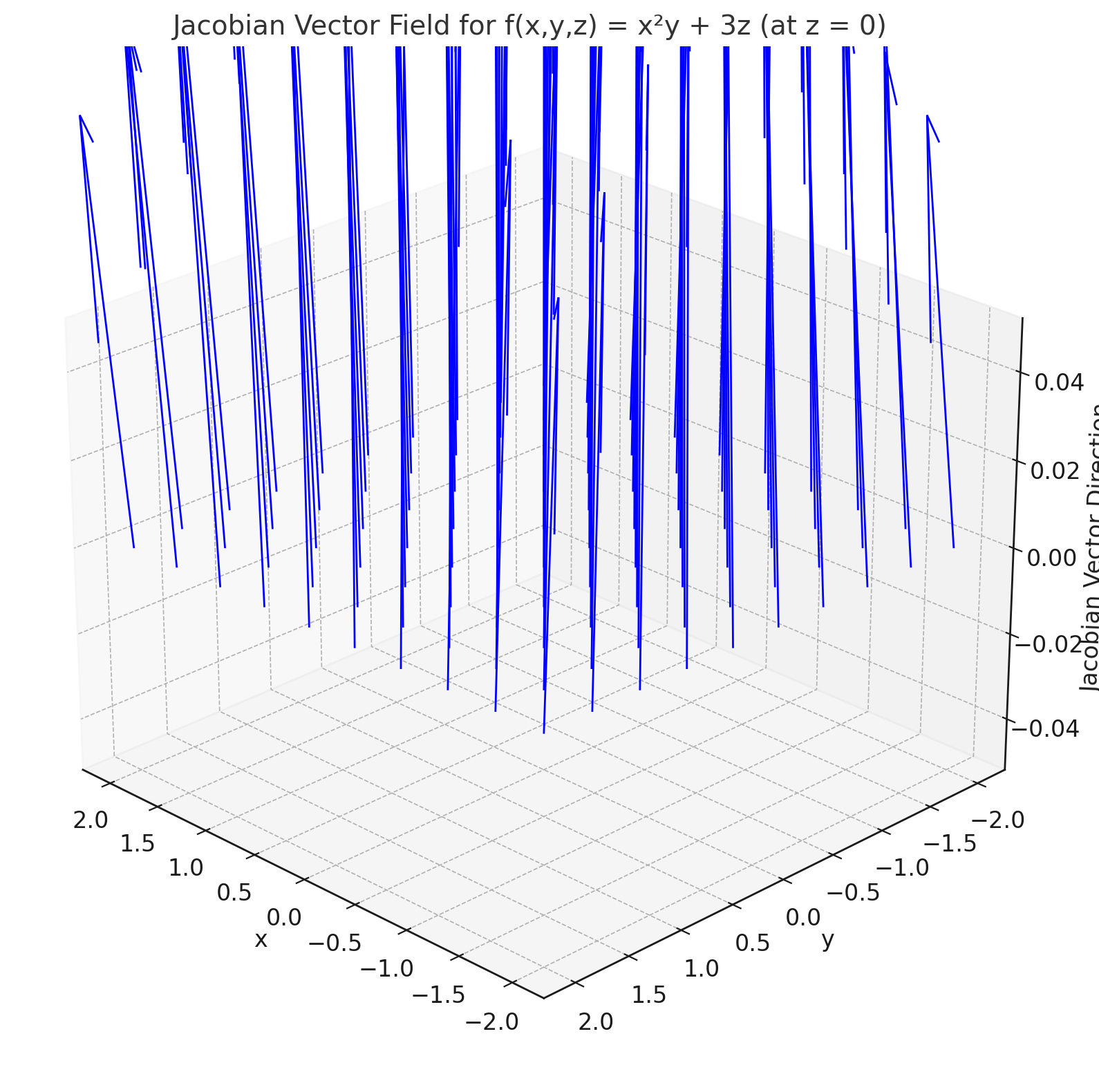
\[ \mathbf{J} = [2xy,\ x^2,\ 3] \]

A 3D plot showing the function ( f(x,y,z) = x^2 y + 3z ), with arrows (vectors) drawn at a few points, pointing in the direction of the gradient. Use one red arrow labeled “Jacobian” pointing toward a steeper slope.

---

🧠 Geometric Interpretation (2D & 3D)

Imagine a function like:

\[ f(x, y) = e^{-(x^2 + y^2)} \]

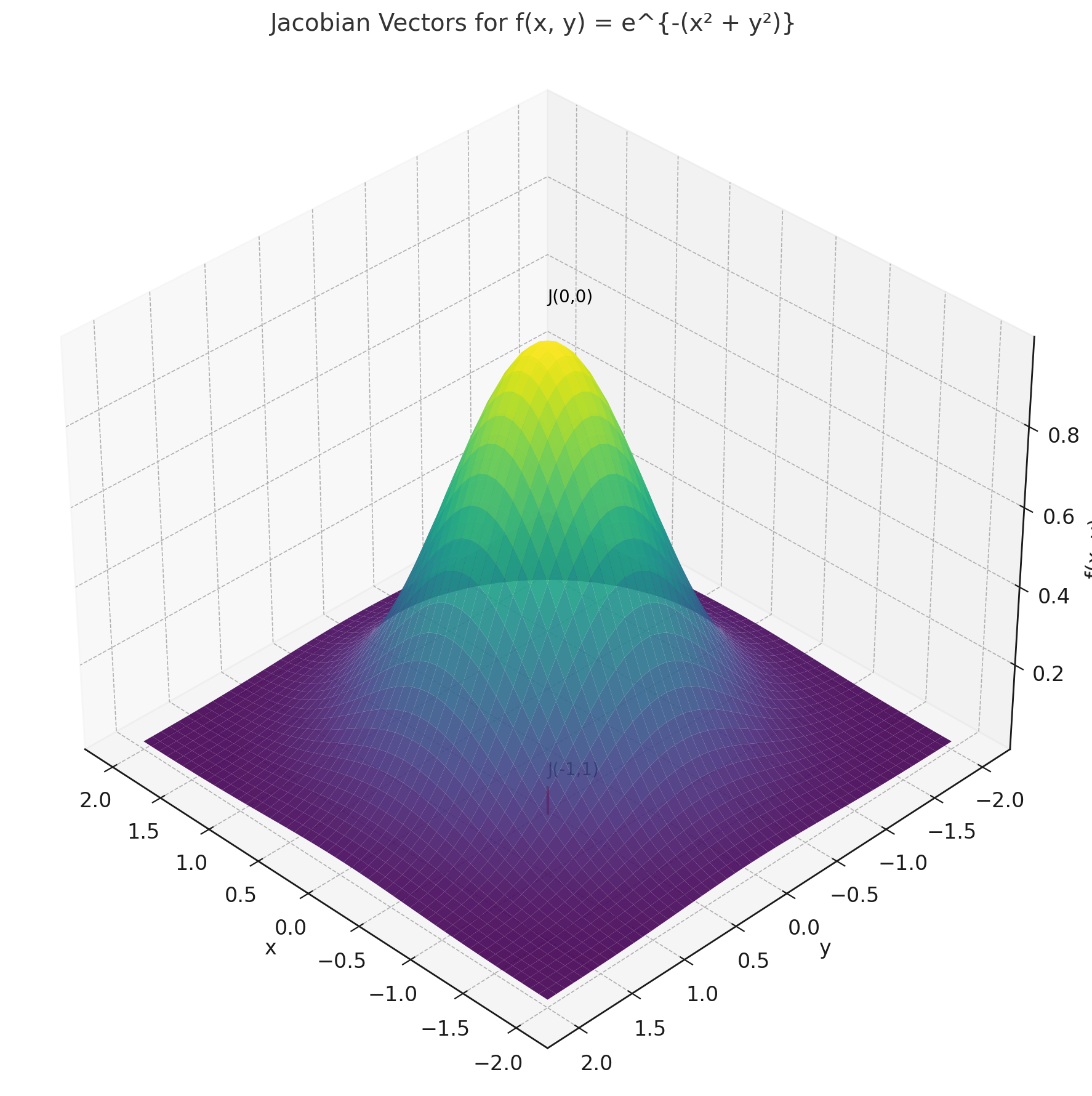
This looks like a hill in 3D — tallest at the center (0, 0), lower as you move out.

Let’s find the Jacobian at specific points.

▶ At point \( (-1, 1) \):

\[ \frac{\partial f}{\partial x} = -2x e^{-(x^2 + y^2)} = -2(-1) e^{-2} ≈ 0.27
\frac{\partial f}{\partial y} = -2y e^{-(x^2 + y^2)} = -2(1) e^{-2} ≈ -0.27
\Rightarrow \mathbf{J}_{(-1, 1)} ≈ [0.27,\ -0.27] \]

▶ At point \( (0, 0) \):

\[ \frac{\partial f}{\partial x} = 0 \quad \frac{\partial f}{\partial y} = 0 \Rightarrow \mathbf{J}_{(0, 0)} = [0,\ 0] \]

✅ Interpretation:

• At the center (0,0), the slope is flat (Jacobian = 0).
• At (-1,1), the vector points from lower to higher elevation — steepest path upward.

A 3D “bell-shaped” surface plot of \( f(x, y) = e^{-(x^2 + y^2)} \) with vectors shown at (-1,1) and (0,0). The (-1,1) point shows a diagonal vector pointing up-right. Label that vector as “Jacobian ≈ [0.27, -0.27]”. At (0,0), show a flat point with a “Jacobian = 0” label.

---

🔁 Jacobian of a Vector-Valued Function (Matrix Form)

When your function returns multiple outputs, the Jacobian becomes a matrix.

Suppose:

\[ u(x, y) = x - 2y \]

\[v(x, y) = 3y - 2x \]

You want the Jacobian matrix \( J(x, y) \), where:

\[ J = \begin{bmatrix} \frac{\partial u}{\partial x} & \frac{\partial u}{\partial y}
\frac{\partial v}{\partial x} & \frac{\partial v}{\partial y} \end{bmatrix} \]

✅ Solving:

• \( \frac{\partial u}{\partial x} = 1 \quad \frac{\partial u}{\partial y} = -2 \)
• \( \frac{\partial v}{\partial x} = -2 \quad \frac{\partial v}{\partial y} = 3 \)

So:

\[ J(x, y) = \begin{bmatrix} 1 & -2
-2 & 3 \end{bmatrix} \]

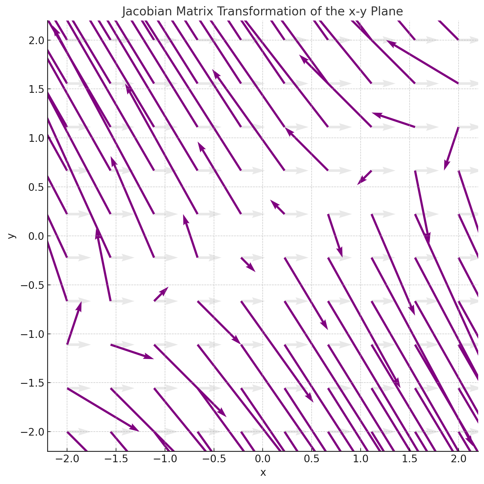
✅ This matrix tells how the output vector \( [u(x,y),\ v(x,y)] \) changes with small changes in \( x, y \).

---

🤖 Relevance to Machine Learning

The Jacobian plays a major role in many ML and deep learning workflows:

• Gradient-Based Optimization: Jacobians are used in calculating gradients during training (e.g., gradient descent).
• Backpropagation: In neural networks, the chain rule involves Jacobians to propagate errors layer by layer.
• Feature Sensitivity: Jacobians help us understand how sensitive outputs are to each input variable.
• Autoencoders & Manifold Learning: Used to study how input spaces are warped/compressed by nonlinear layers.
• Robustness & Adversarial Attacks: Jacobians help compute perturbations that can fool models.
• Jacobian Regularization: Some models penalize extreme Jacobians to improve generalization or smoothness.

---

🧠 Level Up

• 💥 Multivariate Chain Rule: Jacobians are essential for combining nested vector functions.
• 🧠 Neural Networks: Jacobians appear during backpropagation and sensitivity analysis.
• 📈 Optimization: The Jacobian is key in gradient descent, Newton’s method, and convergence analysis.
• 🧮 Change of Variables in Integrals: Jacobian determinants appear when switching coordinate systems (e.g., Cartesian to polar).
• 🎯 Jacobian Determinant: If the determinant ≠ 0, the transformation is locally invertible (used in system stability and transformations).

---

✅ Best Practices

• 📊 Always check your function type: Is it scalar → vector Jacobian? Or vector → matrix Jacobian?
• 🔁 Use partial derivatives systematically: Label each one carefully and check dimensions.
• 🧠 Visualize in 2D or 3D: Understand what the Jacobian vector/matrix tells you about direction and magnitude.
• 🧮 Evaluate at specific points: If analyzing behavior locally, plug in real numbers.
• 🧰 Use symbolic tools: Use Python (`sympy`), WolframAlpha, or MATLAB to verify partials.
• 📐 Think geometry: Jacobian vectors point uphill. Jacobian matrices bend space.

---

⚠️ Common Pitfalls

• ❌ Confusing gradient with output: The Jacobian of a scalar function is a **vector</b>, not a scalar.
• ❌ Mixing vector and matrix Jacobians: Scalar-valued functions → vector (gradient), vector-valued functions → matrix.
• ❌ Skipping zero derivatives: Even if a variable doesn’t show up in one term, still compute its partial.
• ❌ Forgetting evaluation point: The Jacobian changes depending on where you evaluate it. Don't treat it as constant.
• ❌ Ignoring visualization: Without imagining the geometry (direction/slope), it's easy to lose intuition.

---

📌 Try It Yourself

📊 Vector Jacobian: What is the Jacobian vector for \( f(x, y, z) = \sin(xy) + z^2 \) ?

🧠 Step-by-step:
- \( \frac{\partial f}{\partial x} = y \cdot \cos(xy) \)
- \( \frac{\partial f}{\partial y} = x \cdot \cos(xy) \)
- \( \frac{\partial f}{\partial z} = 2z \)
✅ Final Answer: \[ \mathbf{J} = [y \cos(xy),\ x \cos(xy),\ 2z] \]

---

📊 Evaluate at a Point: Find the Jacobian of \( f(x, y) = \ln(x^2 + y^2) \) at \( (1, 2) \)

🧠 Step-by-step:
- \( \frac{\partial f}{\partial x} = \frac{2x}{x^2 + y^2} \)
- \( \frac{\partial f}{\partial y} = \frac{2y}{x^2 + y^2} \) At \( (1, 2) \), the denominator becomes \( 1 + 4 = 5 \)
✅ Final Answer: \[ \mathbf{J}_{(1,2)} = \left[ \frac{2}{5},\ \frac{4}{5} \right] \]

---

📊 Jacobian Matrix: Given:
\( u(x, y) = x^2 + y \),
\( v(x, y) = y^2 - x \), find the Jacobian matrix \( J(x, y) \).

🧠 Step-by-step:
- \( \frac{\partial u}{\partial x} = 2x \), \( \frac{\partial u}{\partial y} = 1 \)
- \( \frac{\partial v}{\partial x} = -1 \), \( \frac{\partial v}{\partial y} = 2y \)

✅ Final Answer: \[ J(x, y) = \begin{bmatrix} 2x & 1 \\ -1 & 2y \end{bmatrix} \]

---

📊 Visual Thinking: Sketch or imagine the surface of \( f(x, y) = x^2 - y^2 \)

🧠 Hint:
This is a saddle surface — increasing in one direction, decreasing in another. - The Jacobian vector at any point will point toward the direction of steepest increase. - Try visualizing a vector field where arrows point in the gradient direction. ✍️ Try plotting a few gradient vectors by hand or in Python!

---

✅ Summary

Let’s wrap up the key points about Jacobians:

---

Topic	Summary
Jacobian of scalar function	Vector of partial derivatives → shows steepest ascent direction
Jacobian of vector-valued function	Matrix of partials → tracks how multiple outputs change with inputs
Geometric meaning	Vectors point from low to high regions — visualize slope
Matrix transformation	Jacobian matrix stretches, rotates, or compresses space locally
In machine learning	Used in gradient descent, backpropagation, and feature sensitivity

---

🧠 Mastering Jacobians gives you the tools to understand direction, scale, and curvature in multivariable systems — essential for modern ML models.

---

💬 Got a question or suggestion?

Leave a comment below — I’d love to hear your thoughts or help if something was unclear.

---

🧭 Next Up

Now that you’ve learned how to construct and interpret the Jacobian, you’re ready for the next step in multivariable calculus and machine learning: Optimization.

In the upcoming post, we’ll explore:

• How to find critical points using gradients and Hessians
• The role of Jacobian and gradient descent in training ML models
• Visual intuition behind minima, maxima, and saddle points
• How optimization shapes neural networks, regression, and clustering

Stay sharp — you’re about to enter the engine room of how machines learn.