Sampling Distribution of the Sample Proportion
🎯 The Sampling Distribution of the Sample Proportion
In a population, the proportion is the number of successful outcomes over the total number of cases. This proportion is denoted by \( \beta \).
For a sample, the proportion is represented by \( p \), which is an estimate of \( \beta \) (population proportion). As the sample size increases, \( p \) gets closer to \( \beta \).
- Number of samples = \( N \)
- Sample proportion = \( p \)
📚 This post is part of the "Intro to Statistics" series
🔙 Previously: Population, Sample, and Sampling Distributions Explained
🔍 Example: Proportion of Voters Supporting a Candidate
Imagine you’re conducting a poll to determine the proportion of voters supporting a political candidate in a city. Out of a sample of 1000 people:
- 600 people say they support the candidate, so the sample proportion \( p = \frac{600}{1000} = 0.6 \).
If you repeat this polling process many times, the sample proportions will vary. The more samples you take, the closer \( p \) will get to the\( \beta ), which is the true support rate in the city.
📊 Key Properties of the Sampling Distribution of the Sample Proportion
- As the number of samples approaches infinity, the sample proportion \( p \) will approximate the population proportion \( \beta \).
- The mean of the sampling distribution of the sample proportion is \( \mu_p = \mu \) (the population proportion).
- The sampling distribution is approximately normal if:
- \( n \times \beta \geq 15 \)
- \( n \times (1 - \beta) \geq 15 \)
This is because we are working with binary categorical data, where the outcomes are either “success” or “failure.”
🔎 Conditions for Normality
- The sampling distribution of the sample proportion will be approximately bell-shaped if:
- \( n \times \beta \geq 15 \)
- \( n \times (1 - \beta) \geq 15 \)
Where:
- \( n \) = sample size
- \( \beta \) = population proportion (success rate)
This ensures that the data behaves like a normal distribution and we can use standard statistical tools like Z-scores.
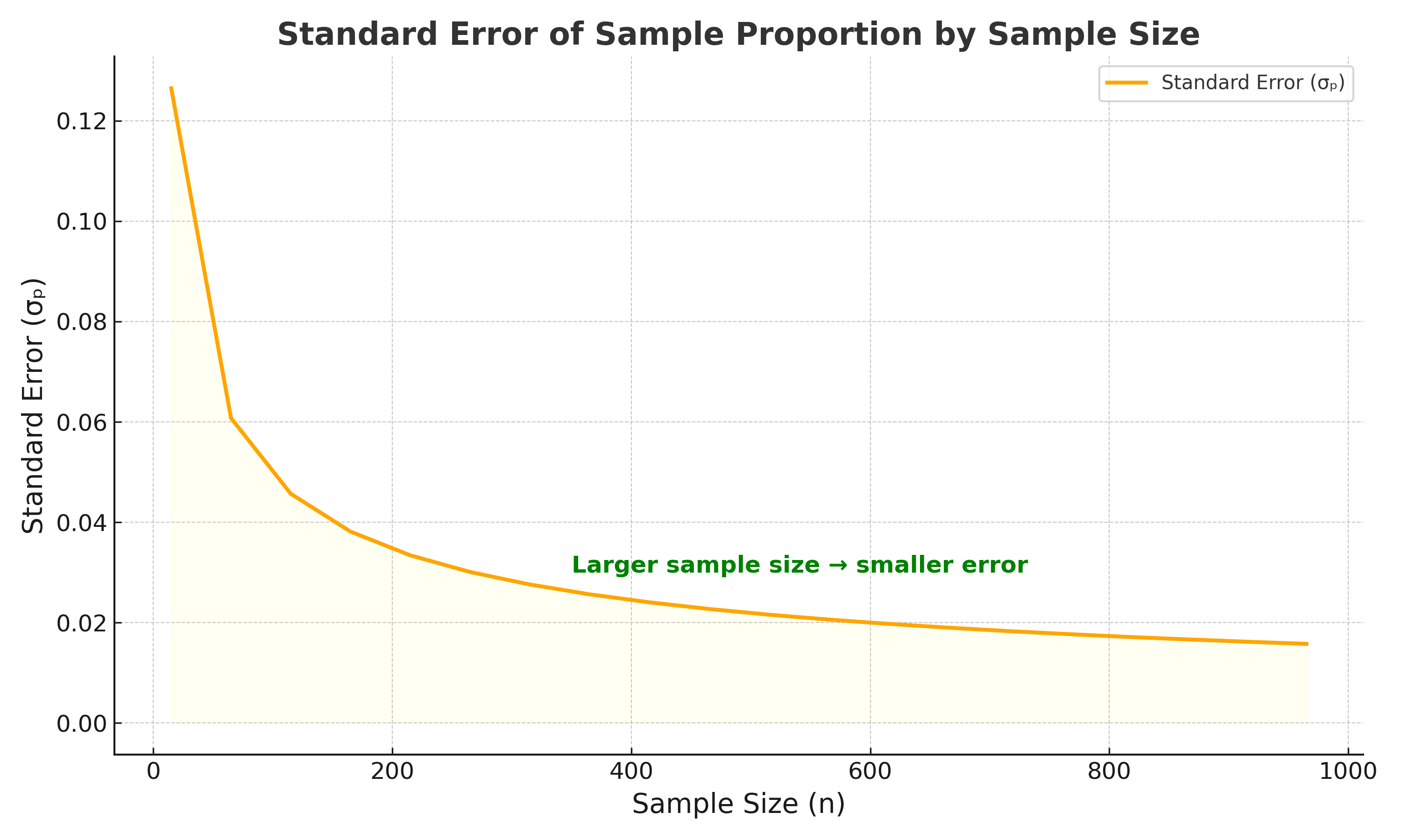
📏 Standard Deviation of the Sample Proportion
The standard deviation (also called the standard error) of the sample proportion is given by the formula:
\[ \sigma_p = \sqrt{\frac{\beta(1 - \beta)}{n}} \]
Where:
- \( \beta \) = population proportion
- \( n \) = sample size
Example:
Let’s assume a population proportion of \( \beta = 0.6 \) (60% of people support a candidate), and you take a sample of size \( n = 1000 \).
The standard error is:
\[ \sigma_p = \sqrt{\frac{0.6(1 - 0.6)}{1000}} = \sqrt{\frac{0.24}{1000}} = 0.0155 \]
This means the sample proportion will vary by about 0.0155 from the true population proportion on average.
⚖️ Calculating Proportions for Binary Categorical Variables
When dealing with binary categorical variables (like success/failure, yes/no), we don’t need to calculate the mean or standard deviation using traditional methods. Instead, we compute the proportion \( \beta \) for the population and \( p \) for the sample.
- Population Proportion \( \beta \)
- Sample Proportion \( p \)
- Standard Deviation of the sample proportion \( \sigma_p \)
Example:
- Population: 60% support the candidate (\( \beta = 0.6 \))
- Sample: 550 out of 1000 support the candidate (\( p = 0.55 \))
Use the formula to find the standard error for further analysis.
🧠 Level Up: Advanced Insights on Sampling Proportions
- The Central Limit Theorem ensures that as the sample size increases, the sampling distribution of the sample proportion becomes approximately normal, allowing for easier statistical inference.
- When sample size \( n \) is large enough (usually \( n \geq 30 \)) and both \( n\beta \geq 15 \) and \( n(1-\beta) \geq 15 \) hold, the sampling distribution of the sample proportion will follow a normal distribution.
- To improve accuracy, confidence intervals and hypothesis tests can be applied to sample proportions, leveraging the normality assumption from the CLT.
- If the sample size is small or the conditions for normality aren’t met, other techniques like binomial approximation or bootstrapping can be used for more reliable results.
✅ Best Practices for Proportional Sampling
- Ensure your sample size is large enough so that
n × β ≥ 15andn × (1 - β) ≥ 15. - Use random and representative sampling to reduce bias in estimating
p. - Report a confidence interval with your sample proportion for better interpretation.
- Verify that your variable is binary (success/failure) before applying this model.
⚠️ Common Pitfalls to Avoid
- ❌ Applying the normal approximation when
n × βorn × (1 - β)is less than 15. - ❌ Misinterpreting
pas a fixed value — it's a random variable. - ❌ Forgetting that standard deviation decreases with larger samples.
- ❌ Confusing the population proportion
βwith the sample proportionp.
📌 Try It Yourself: Sampling Proportions
Q1: What does the sampling distribution of the sample proportion represent?
💡 Show Answer
- A) Distribution of sample proportions from many samples ✓
- B) Distribution of individual data points in the population
- C) Distribution of population proportions
- D) Distribution of standard errors
Q2: What is the central limit theorem's role in sampling distributions?
💡 Show Answer
- A) It states that the sample means follow a normal distribution, regardless of the population distribution ✓
- B) It ensures that larger sample sizes always lead to non-normal distributions
- C) It calculates the proportion of successes in the population
- D) It assumes all population distributions are normally distributed
Q3: In the formula for the standard error of the sample proportion, what does \( n \) represent?
💡 Show Answer
- A) The population size
- B) The sample size ✓
- C) The proportion of successes
- D) The standard deviation of the population
Q4: For the sampling distribution of the sample proportion to be approximately normal, which condition must hold?
💡 Show Answer
- A) \( n \times \beta \geq 15 \) and \( n \times (1 - \beta) \geq 15 \) ✓
- B) \( n \times \beta \geq 10 \) and \( n \times (1 - \beta) \geq 10 \)
- C) \( n \geq 50 \)
- D) The population proportion \( \beta \) must be 0.5
Q5: How is the standard deviation (standard error) of the sample proportion calculated?
💡 Show Answer
- A) \( \sigma_p = \frac{\beta(1 - \beta)}{n} \)
- B) \( \sigma_p = \frac{\sigma}{\sqrt{n}} \)
- C) \( \sigma_p = \sqrt{\frac{\beta(1 - \beta)}{n}} \) ✓
- D) \( \sigma_p = \frac{\beta}{n} \)
✅ Summary
| Concept | Description |
|---|---|
| Population Proportion (\( \beta \)) | Proportion of successful outcomes in the population. |
| Sample Proportion (\( p \)) | Proportion of successful outcomes in a sample. |
| Sampling Distribution | Theoretical distribution of sample proportions from many samples |
| Mean of Sampling Distribution | Equals the population proportion \( \mu_p = \mu \) |
| Standard Error (\( \sigma_p \)) | \( \sigma_p = \sqrt{\frac{\beta(1 - \beta)}{n}} \), variability of sample proportions |
| Conditions for Normality | \( n \times \beta \geq 15 \) and \( n \times (1 - \beta) \geq 15 \) for bell-shaped curve. |
🔜 Up Next
In the next post, we’ll explore The Sampling Distribution of the Sample Mean in more detail — how sample averages behave and how to apply them in statistical procedures.
Stay curious! 📈
📺 Explore the Channel

🎥 Hoda Osama AI
Learn statistics and machine learning concepts step by step with visuals and real examples.
💬 Got a Question?
Leave a comment or open an issue on GitHub — I love connecting with other learners and builders. 🔁