Mean, Variance, and Standard Deviation of Random Variables
How do we summarize a random variable with a single number?
What happens to the mean and variance if we shift or scale the variable?
This post explains the mean, variance, and standard deviation for both discrete and continuous random variables — with concrete examples.
📚 This post is part of the "Intro to Statistics" series
🔙 Previously: What Are Random Variables and How Do We Visualize Their Distributions?
📏 What Is the Mean of a Random Variable?
The mean (or expected value) of a random variable ( X ) is its probability-weighted average of all possible values.
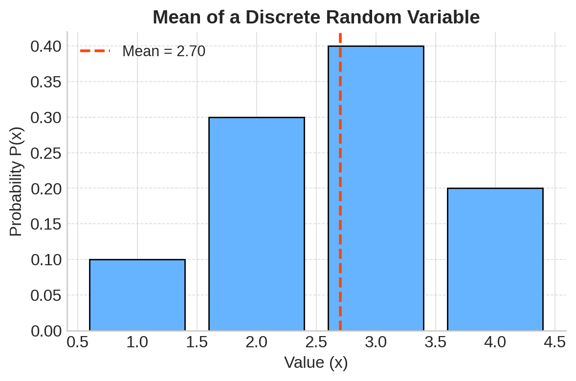
🧮 Mean of a Discrete Random Variable
\[ \mu_X = E(X) = \sum_i x_i P(x_i) \]
This means each value \( x_i \) is weighted by its probability \( P(x_i) \).
Example:
| \(x_i\) | 1 | 2 | 3 | 4 |
|---|---|---|---|---|
| \(P(x_i)\) | 0.1 | 0.3 | 0.4 | 0.2 |
Calculate:
\[ E(X) = 1 \times 0.1 + 2 \times 0.3 + 3 \times 0.4 + 4 \times 0.2 = 0.1 + 0.6 + 1.2 + 0.8 = 2.7 \]
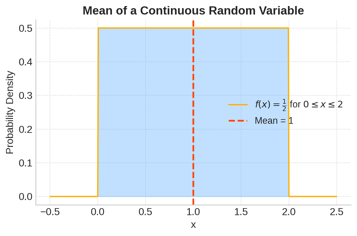
📐 Mean of a Continuous Random Variable
\[ \mu_X = E(X) = \int_{-\infty}^{\infty} x f(x) \, dx \]
Where \( f(x) \) is the probability density function (PDF).
Example:
If
\[ f(x) = \frac{1}{2} \quad \text{for } 0 \leq x \leq 2, \quad 0 \text{ otherwise} \]
Then
\[ E(X) = \int_0^2 x \times \frac{1}{2} \, dx = \frac{1}{2} \int_0^2 x \, dx = \frac{1}{2} \times \left[ \frac{x^2}{2} \right]_0^2 = \frac{1}{2} \times 2 = 1 \]
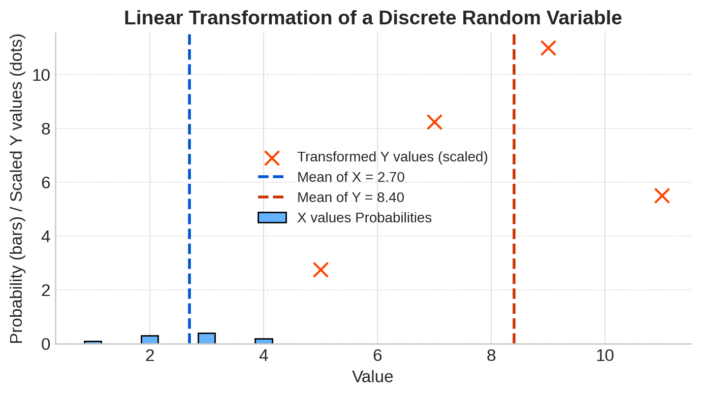
🔄 Mean Under Linear Transformations
If we transform \( X \) as:
\[ Y = a + bX \]
then
\[ E(Y) = a + b E(X) \]
Example (Using discrete mean above):
\[ E(Y) = 3 + 2 \times 2.7 = 3 + 5.4 = 8.4 \]
📊 What Is Variance?
Variance measures the spread or deviation of values around the mean:
\[ \text{Var}(X) = E[(X - \mu)^2] \]
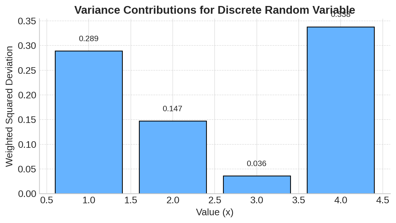
🧮 Variance for Discrete Random Variable
\[ \text{Var}(X) = \sum_i (x_i - \mu)^2 P(x_i) \]
Using the discrete example above (\( \mu = 2.7 \)):
\[ \text{Var}(X) = (1 - 2.7)^2 \times 0.1 + (2 - 2.7)^2 \times 0.3 + (3 - 2.7)^2 \times 0.4 + (4 - 2.7)^2 \times 0.2 \]
\[ = (2.89)(0.1) + (0.49)(0.3) + (0.09)(0.4) + (1.69)(0.2) \]
\[ = 0.289 + 0.147 + 0.036 + 0.338 \]
\[ = 0.81 \]
📐 Variance for Continuous Random Variable
\[ \text{Var}(X) = \int_{-\infty}^\infty (x - \mu)^2 f(x) \, dx \]
For the continuous example above (\( \mu=1 \)):
\[ \text{Var}(X) = \int_0^2 (x - 1)^2 \times \frac{1}{2} \, dx = \frac{1}{2} \int_0^2 (x^2 - 2x + 1) \, dx \]
Calculate:
\[ = \frac{1}{2} \left[ \frac{x^3}{3} - x^2 + x \right]_0^2 = \frac{1}{2} \left( \frac{8}{3} - 4 + 2 \right) = \frac{1}{2} \times \frac{2}{3} = \frac{1}{3} \approx 0.333 \]
🔄 Variance Under Linear Transformations
For \( Y = a + bX \), variance changes as:
\[ \text{Var}(Y) = b^2 \text{Var}(X) \]
Adding or subtracting a constant \( a \) does not affect variance.
✏️ Proof Sketch:
\[ \text{Var}(Y) = E[(Y - E[Y])^2] \]
\[ = E[(a + bX - (a + bE[X]))^2] \]
\[ = E[(b(X - E[X]))^2] \]
\[ = b^2 E[(X - E[X])^2] \]
\[ = b^2 \text{Var}(X) \]
Example:
Using previous discrete variance ( 0.81 ):
\[ \text{Var}(Y) = 2^2 \times 0.81 = 4 \times 0.81 = 3.24 \]
📏 Standard Deviation and Scaling
Standard deviation \( \sigma \) is the square root of variance:
\[ \sigma_X = \sqrt{\text{Var}(X)} \]
For \( Y = a + bX \):
\[ \sigma_Y = \sqrt{\text{Var}(Y)} = \sqrt{b^2 \text{Var}(X)} = |b| \sigma_X \]
Example (continued):
\[ \sigma_X = \sqrt{0.81} = 0.9 \]
\[ \sigma_Y = 2 \times 0.9 = 1.8 \]
🔢 Variance of Sum and Difference
For any two variables \( X \) and \( Y \):
\[ \text{Var}(X \pm Y) = \text{Var}(X) + \text{Var}(Y) \pm 2\,\text{Cov}(X, Y) \]
🤖 Why It Matters for Machine Learning
Understanding expected value and variance is foundational to many machine learning algorithms:
- 📊 Feature Scaling: When features are transformed (e.g., using standardization or min-max scaling), you're applying linear transformations — and knowing how these affect mean and variance helps you avoid introducing bias.
- 🧠 Loss Functions: Common losses like
MSErely on variance concepts — minimizing variance between predicted and actual values improves model performance. - 📈 Model Interpretation: Many models assume data has constant variance (homoscedasticity). Violating this can lead to poor generalization.
💡 Mastering these statistical fundamentals makes it easier to debug models, improve feature engineering, and better understand algorithm behavior under the hood.
🧠 Level Up: Understanding Variance Properties
✅ Best Practices for Working with Random Variable Metrics
- Always check whether your variable is discrete or continuous before choosing formulas.
- Use linear transformation rules to simplify calculations and scaling checks.
- Understand that standard deviation is more interpretable in the context of units.
- Apply variance rules carefully when dealing with sums of variables.
⚠️ Common Pitfalls to Avoid
- ❌ Confusing the formula for variance between sample vs. population.
- ❌ Forgetting to square the scaling factor when applying transformations to variance.
- ❌ Assuming that adding constants affects the variance (it doesn’t).
- ❌ Neglecting covariance when computing variance of sums.
📌 Try It Yourself: Mean, Variance & Linear Transformations
Q1: What does the expected value (mean) of a discrete random variable represent?
💡 Show Answer
✅ It’s the probability-weighted average of all possible outcomes.
In other words, it's the long-run average value you’d expect over many trials.
Q2: For a linear transformation \( Y = a + bX \), how do you compute the expected value \( E(Y) \)?
💡 Show Answer
✅ \( E(Y) = a + b \cdot E(X) \)
This means the expected value shifts and scales along with the transformation.
Q3: If you add a constant \( a \) to every value of a random variable, how does it affect the variance?
💡 Show Answer
✅ It doesn’t change the variance.
Variance only measures spread, not the location — adding a constant shifts all values equally.
Q4: For \( Y = a + bX \), how is the variance of \( Y \) related to the variance of \( X \)?
💡 Show Answer
✅ \( \text{Var}(Y) = b^2 \cdot \text{Var}(X) \)
Because scaling a variable by \( b \) increases the spread by \( b^2 \), while the constant \( a \) has no effect.
✅ Summary
| Concept | Formula / Description |
|---|---|
| Mean (Discrete) | \( \mu = \sum x_i P(x_i) \) |
| Mean (Continuous) | \( \mu = \int x f(x) dx \) |
| Variance (Discrete) | \( \sigma^2 = \sum (x_i - \mu)^2 P(x_i) \) |
| Variance (Continuous) | \( \sigma^2 = \int (x - \mu)^2 f(x) dx \) |
| Linear Transform Mean | \( E(a + bX) = a + b E(X) \) |
| Linear Transform Variance | \( \text{Var}(a + bX) = b^2 \text{Var}(X) \) |
| Variance of Sum/Diff | \( \text{Var}(X \pm Y) = \text{Var}(X) + \text{Var}(Y) \pm 2\text{Cov}(X,Y) \) |
| Std Deviation | \( \sigma = \sqrt{\text{Var}(X)} \) |
🔜 Up Next
Next, we’ll explore the Normal Distribution — a fundamental continuous distribution that appears everywhere in statistics and data science.
Stay tuned!
📺 Explore the Channel

🎥 Hoda Osama AI
Learn statistics and machine learning concepts step by step with visuals and real examples.
💬 Got a Question?
Leave a comment or open an issue on GitHub — I love connecting with other learners and builders. 🔁