🔁 From Limits to Smoothness: Transformations, Limits, Continuity & Differentiability

🔁 Functions as Transformations

A function can be seen as a machine: it takes input values and returns output values. But in a more visual and geometric sense, a function can be thought of as a transformation — changing or warping the input space into a new shape.

---

📚 This post is part of the "Intro to Calculus" series

🔙 Previously: Visualizing Multivariable Functions: Contour Plots, Vector-Valued Functions & Vector Fields (Beginner's Guide)

🔜 Next: What is a Derivative? (Beginner’s Guide to Calculus for ML)

---

📚 Mathematical Idea

If we start with a point \( x \in \mathbb{R} \), a function \( f(x) \) maps it to another real number \( y \).
For a 2D transformation:

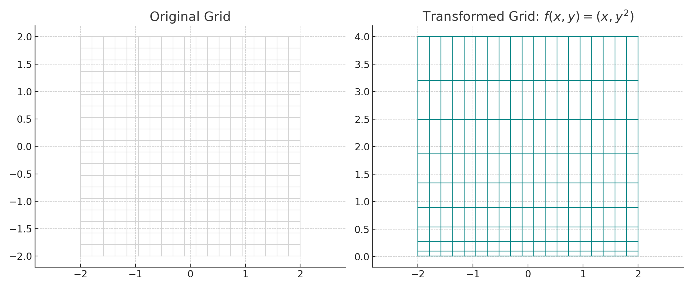
\[ f(x, y) = (x, y^2) \]

This “bends” the coordinate plane vertically — keeping \( x \) unchanged but squaring the \( y \)-coordinate.

🧪 Python Example: Transforming a Grid

Visual: Show a grid before and after the transformation \( f(x, y) = (x, y^2) \)

import numpy as np
import matplotlib.pyplot as plt

x, y = np.meshgrid(np.linspace(-2, 2, 20), np.linspace(-2, 2, 20))
x_new = x
y_new = y ** 2

fig, axs = plt.subplots(1, 2, figsize=(10, 4))
axs[0].quiver(x, y, np.zeros_like(x), np.zeros_like(y), color='gray')
axs[0].set_title("Original Grid")
axs[0].axis('equal')

axs[1].quiver(x_new, y_new, np.zeros_like(x), np.zeros_like(y), color='teal')
axs[1].set_title("Transformed Grid: $f(x, y) = (x, y^2)$")
axs[1].axis('equal')

plt.tight_layout()
plt.show()

---

Left panel shows the original 2D grid. Right panel shows how the transformation bends the grid vertically, curving the 𝑦 y-coordinates upward while preserving the 𝑥 x-axis.

---

📉 What Is a Limit?

A limit describes what a function is approaching as the input gets closer and closer to a specific value — even if the function is not defined at that value.

📚 Mathematical Definition

\[ \lim_{x \to a} f(x) = L \]

This means: as \( x \) gets arbitrarily close to \( a \), the value of \( f(x) \) gets arbitrarily close to \( L \).

🔍 Example:

Let:

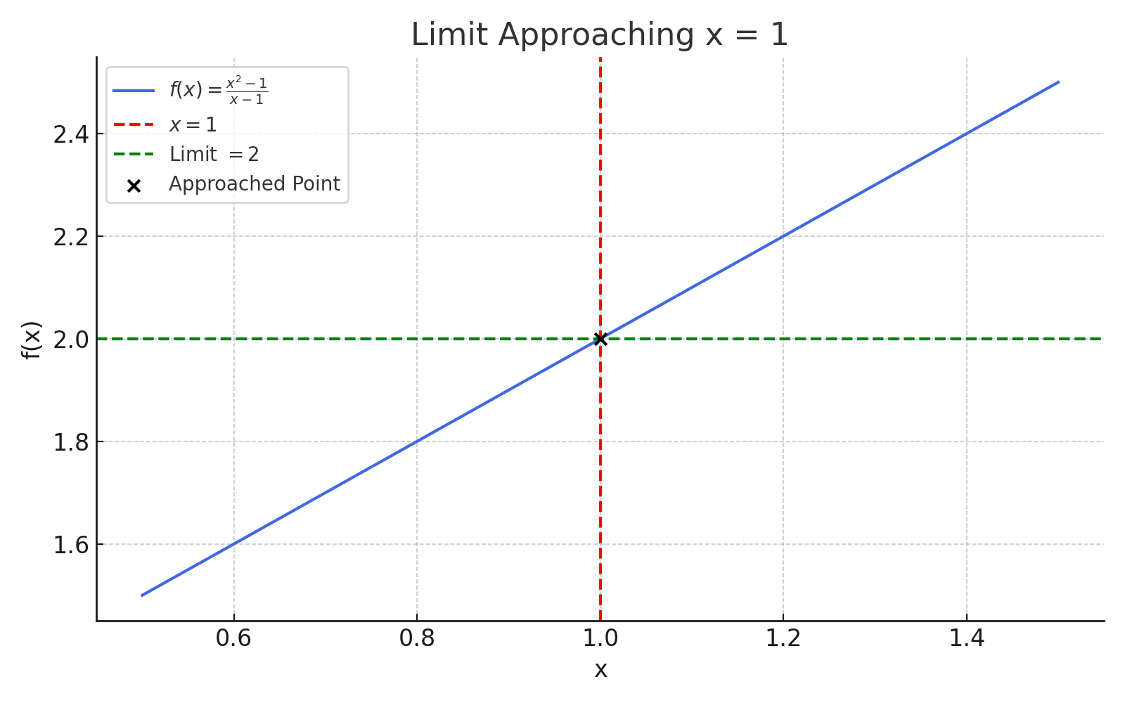
\[ f(x) = \frac{x^2 - 1}{x - 1} \]

At \( x = 1 \), the function is undefined — but we can factor:

\[ f(x) = \frac{(x - 1)(x + 1)}{x - 1} = x + 1 \quad \text{(for } x \neq 1 \text{)} \]

So:

\[ \lim_{x \to 1} f(x) = 2 \]

🧪 Python Visualization

x = np.linspace(0.5, 1.5, 200)
y = (x**2 - 1)/(x - 1)

plt.plot(x, y, label=r'$f(x) = \frac{x^2 - 1}{x - 1}$')
plt.axvline(1, color='red', linestyle='--', label='x = 1')
plt.axhline(2, color='green', linestyle='--', label='Limit = 2')
plt.xlabel('x')
plt.ylabel('f(x)')
plt.title('Limit Approaching x = 1')
plt.legend()
plt.grid(True)
plt.show()

---

---

🧩 Examples of Limits in Functions

🔹 One-Sided Limits

\[ \lim_{x \to a^-} f(x) \quad \text{and} \quad \lim_{x \to a^+} f(x) \]

The full limit exists only when both sides agree.

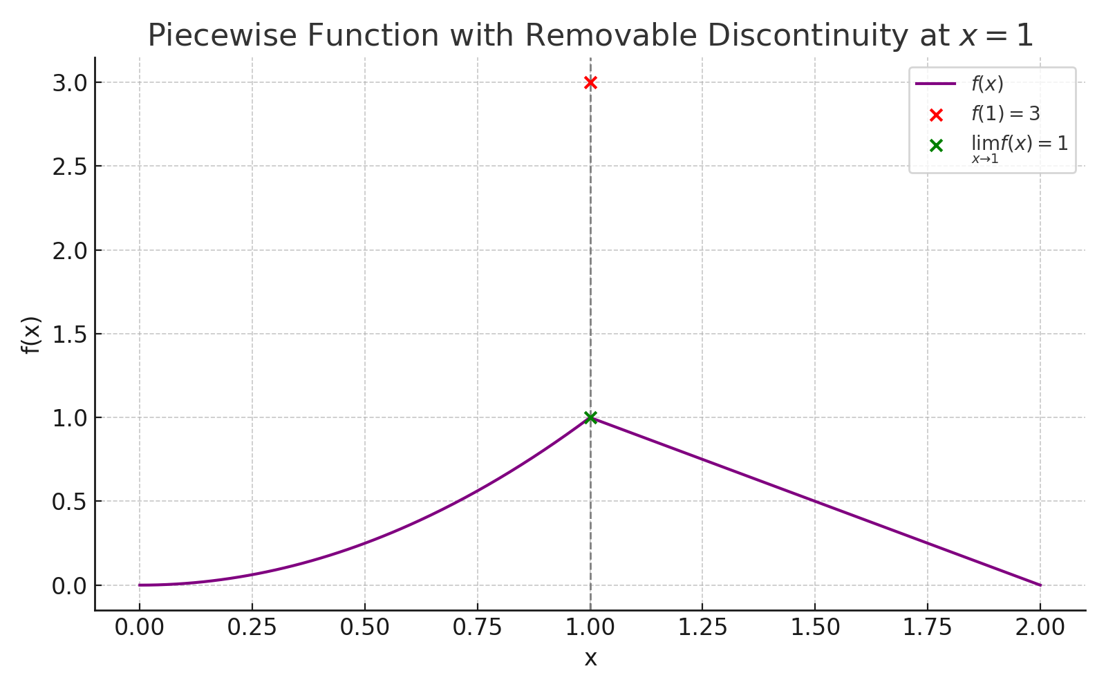
🔹 Piecewise Example:

\[ f(x) = \begin{cases} x^2 & \text{if } x < 1 \ 3 & \text{if } x = 1 \ 2 - x & \text{if } x > 1 \end{cases} \]

Then:

\[ \lim_{x \to 1^-} f(x) = 1 \quad \text{and} \quad \lim_{x \to 1^+} f(x) = 1 \Rightarrow \lim_{x \to 1} f(x) = 1 \]

But:

\[ f(1) = 3 \neq \lim_{x \to 1} f(x) \]

So the function has a removable discontinuity at \( x = 1 \).

---

—

🔗 Continuity and Differentiability

✅ Continuity

A function \( f(x) \) is continuous at \( x = a \) if:

1. \( f(a) \) is defined
2. \( \lim_{x \to a} f(x) \) exists
3. \( \lim_{x \to a} f(x) = f(a) \)

✅ Differentiability

A function is differentiable at \( x = a \) if it is continuous and smooth (no sharp corners or cusps).

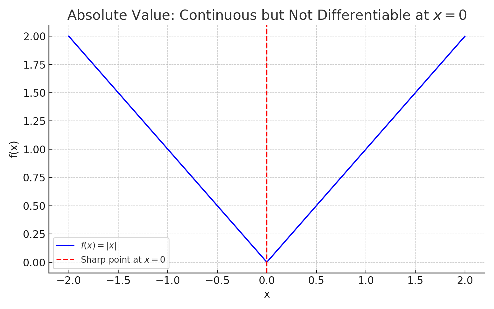
🔍 Example: \( f(x) = |x| \)

• Continuous everywhere
• Not differentiable at \( x = 0 \) because of a sharp point

🧪 Python Visualization

x = np.linspace(-2, 2, 400)
y = np.abs(x)

plt.plot(x, y, label=r'$f(x) = |x|$', color='blue')
plt.axvline(0, color='red', linestyle='--', label='x = 0')
plt.xlabel('x')
plt.ylabel('f(x)')
plt.title('Absolute Value: Continuous but Not Differentiable at x = 0')
plt.legend()
plt.grid(True)
plt.show()

---

---

🤖 Relevance to Machine Learning

Understanding limits, continuity, and differentiability is essential for many foundational ideas in machine learning and deep learning:

• 🧠 Gradient Descent & Optimization
  Most learning algorithms (like gradient descent) rely on functions being continuous and differentiable so we can compute smooth gradients to minimize loss.

• 🔁 Backpropagation
  Neural networks use the chain rule to propagate error gradients backward — which requires differentiable activation functions and loss functions.

• 📉 Loss Surfaces
  The cost or loss function must be smooth and continuous for optimizers to navigate toward minima efficiently. Sharp discontinuities can trap or mislead optimization.

• 🧩 Activation Functions
  Common activations (ReLU, sigmoid, tanh) are chosen based on their continuity and differentiability — affecting both model capacity and training dynamics.

• 📐 Regularization & Generalization
  Techniques like L2 regularization implicitly promote smoother (more continuous and differentiable) functions, which helps with generalization and avoiding overfitting.

• ⚠️ Adversarial Robustness
  Discontinuous or non-differentiable spots in the model behavior can be exploited by adversarial examples. Smoothness leads to more stable and robust models.

---

🧭 Key Insight: If your model isn’t differentiable, gradient-based learning breaks down. Smoothness isn’t just elegant — it’s essential!

---

🧠 Level Up

• 🔄 Functions as Mappings: Think of every function as a way to reshape input space — this is crucial for understanding transformations in deep learning layers.
• 📏 Limits and Precision: Mastering limits builds your intuition for numerical stability, convergence, and approximation in ML algorithms.
• 📐 Continuity in Practice: Continuous loss functions ensure smooth training. Discontinuities can cause sudden optimization failures.
• 🧮 Differentiability = Learnability: If a function isn’t differentiable, gradient-based methods (like backpropagation) won’t work.
• 📉 Piecewise Behavior: Recognize when piecewise models like ReLU introduce non-differentiable points — and how this affects learning speed.
• 🧩 Function Smoothness: Smooth, continuous, and differentiable models generalize better and are more robust to noisy data.

---

✅ Best Practices

• 📌 Clearly define your domain: Before analyzing limits or continuity, specify where the function is defined and what happens near edges.
• 🔍 Check one-sided limits: Always test left-hand and right-hand limits — especially for piecewise or discontinuous functions.
• 📉 Use simple plots for intuition: Visualizing limits or corners (like in \(|x|\)) makes differentiability easier to grasp.
• 🧮 Simplify before evaluating: Use algebra (factoring, cancelling) to rewrite functions when limits seem undefined.
• 🧠 Distinguish continuity from differentiability: Remember, a function can be continuous but not differentiable.
• 💡 Test critical points: Especially around \(x = 0\), corners, or undefined values — those are the hotspots for discontinuity or non-smooth behavior.

---

⚠️ Common Pitfalls

• ❌ Assuming all functions are smooth: Not all continuous functions are differentiable. Don’t confuse them.
• ❌ Forgetting removable discontinuities: A function might have a limit even when it’s undefined at a point.
• ❌ Using only numeric evaluation: Relying only on plotting or calculators can miss underlying structure — combine with algebra.
• ❌ Overlooking piecewise definitions: For functions defined in parts, always check each region separately.
• ❌ Ignoring symmetry: Functions like even/odd functions or absolute values have special properties that affect continuity and smoothness.

---

📌 Try It Yourself

📉 Limit Challenge: What is \(\displaystyle \lim_{x \to 2} \frac{x^2 - 4}{x - 2} \) ?

🧠 Step-by-step:
- Factor numerator: \( x^2 - 4 = (x - 2)(x + 2) \)
- Cancel terms: \( \frac{(x - 2)(x + 2)}{x - 2} = x + 2 \) (for \( x \ne 2 \))
✅ Final Answer: \[ \lim_{x \to 2} \frac{x^2 - 4}{x - 2} = 4 \]

---

📈 Continuity Check: Is the function \[ f(x) = \begin{cases} x^2 & x < 1 \\\\ 3 & x = 1 \\\\ 2 - x & x > 1 \end{cases} \] continuous at \( x = 1 \) ?

🧠 Step-by-step:
- Left-hand limit: \( \lim_{x \to 1^-} f(x) = 1^2 = 1 \)
- Right-hand limit: \( \lim_{x \to 1^+} f(x) = 2 - 1 = 1 \)
- But \( f(1) = 3 \) 🤔
❌ Not continuous! ✅ Final Answer: \[ \lim_{x \to 1} f(x) = 1 \ne f(1) \]

---

📐 Differentiability Test: Is \( f(x) = |x| \) differentiable at \( x = 0 \)?

🧠 Hint:
- Left-hand derivative: \( f'(x) = -1 \)
- Right-hand derivative: \( f'(x) = 1 \)
❌ Derivatives don't match at \( x = 0 \), so not differentiable! ✅ Final Answer: \[ f(x) = |x| \text{ is not differentiable at } x = 0 \]

---

🌐 Transformation Intuition: What does \( f(x, y) = (x, y^2) \) do to the plane?

🧠 Insight:
- Keeps \( x \) the same - Squashes negative \( y \) to positive - Bends the grid into a parabolic shape ✅ Visualization: - Try plotting the grid with original vs transformed coordinates!

---

✅ Summary

Let’s wrap up the key ideas from this post:

---

Topic	Summary
Function as Transformation	Warping or reshaping input space — e.g., \( f(x, y) = (x, y^2) \) folds the plane
Limits	Describe how a function behaves near a point — not just at it
Continuity	Function is continuous if limit exists and matches the value at the point
Differentiability	Smoothness — function must have a well-defined slope (no corners)
Relevance to ML	Essential for gradients, backpropagation, and smooth training

---

💬 Got a question or suggestion?

Leave a comment below — I’d love to hear your thoughts or help if something was unclear.

---

🧭 Next Up

Now that you’ve explored how functions behave through transformations, limits, and smoothness, it’s time to zoom in on how they change — and how we measure that change precisely.

In the upcoming post, we’ll dive into:

• What a gradient really is — and how it generalizes the derivative to higher dimensions
• The meaning of instantaneous rate of change in both math and machine learning
• How limits give rise to derivatives, step by step
• Using gradients for approximation and direction-finding in complex systems
• How to calculate derivatives symbolically and numerically using Python

🧠 These tools are essential for optimization, learning, and understanding the terrain of functions.

Stay tuned — we’re about to unlock the core mechanics of calculus and machine learning!