🌄 Visualizing Multivariable Functions: Contour Plots, Vector-Valued Functions & Vector Fields (Beginner's Guide)
Learn how to visualize and understand contour plots, vector-valued functions, and vector fields with Python code and clear examples. A beginner-friendly guide tying math concepts to machine learning.
🧭 Introduction
In this post, we’ll introduce contour plots, vector-valued functions, and vector fields — three core tools for visualizing the behavior of multivariable functions. These concepts are essential for anyone exploring calculus, physics, or machine learning, as they help you build intuition for how functions behave in more than one dimension.
📚 This post is part of the "Intro to Calculus" series
🔙 Previously: Understanding Functions: The Foundation of Calculus (and Machine Learning!)
🔜 Next: From Limits to Smoothness: Transformations, Limits, Continuity & Differentiability
🗺️ What is a Contour Plot?
A contour plot is a 2D plot showing lines (contours) where a function of two variables ($z = f(x, y)$) has constant values. Imagine a topographic map where each line represents locations with the same elevation — contour plots work the same way for functions!
- Use case: Contour plots are widely used in optimization (visualizing a loss surface), physics (potential fields), and engineering.
📊 Example: Contour Plot of $f(x, y) = x^2 + y^2$
1
2
3
4
5
6
7
8
9
10
11
12
13
14
15
16
17
import numpy as np
import matplotlib.pyplot as plt

x = np.linspace(-3, 3, 100)
y = np.linspace(-3, 3, 100)
X, Y = np.meshgrid(x, y)
Z = X2 + Y2

plt.figure(figsize=(6,5))
contour = plt.contour(X, Y, Z, levels=10, cmap='plasma')
plt.clabel(contour, inline=True, fontsize=8)
plt.xlabel('x')
plt.ylabel('y')
plt.title('Contour Plot of $f(x, y) = x^2 + y^2$')
plt.grid(True)
plt.show()
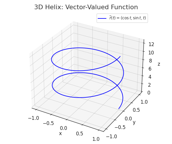
🧭 Vector-Valued Function: Definition & Examples
A vector-valued function produces a vector (more than one number) as an output for each input. If the input is $t$, the output could be $(x(t), y(t))$ — which describes a path or a curve in space.
Real-world analogy: The movement of a particle over time ($t$) can be described as $\vec{r}(t) = (x(t), y(t))$ or in 3D as $(x(t), y(t), z(t))$.
📚 Examples
1. Basic 2D vector-valued function
$\vec{r}(t) = (\cos t, \sin t)$, $t \in [0, 2\pi]$
- This traces out a circle of radius 1.
2. Python Example: Plotting a Circle Path
1
2
3
4
5
6
7
8
9
10
11
12
13
14
15
16
17

import numpy as np
import matplotlib.pyplot as plt

t = np.linspace(0, 2 * np.pi, 100)
x = np.cos(t)
y = np.sin(t)

plt.figure(figsize=(5,5))
plt.plot(x, y, label='$\vec{r}(t) = (\cos t, \sin t)$')
plt.xlabel('x')
plt.ylabel('y')
plt.title('Circle Traced by a Vector-Valued Function')
plt.legend()
plt.axis('equal')
plt.grid(True)
plt.show()
3. Machine Learning Example
Suppose a model predicts both price and rating for a product:
\[\vec{f}(x) = \begin{pmatrix} \text{predicted price}(x) \\ \text{predicted rating}(x) \end{pmatrix}\]- For every input $x$ (product features), the output is a 2D vector.
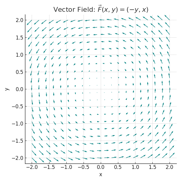
🌪️ What is a Vector Field?
A vector field attaches a vector to every point in a region. It’s like having arrows everywhere showing wind direction and speed at each spot.
Mathematically: $\vec{F}(x, y) = (P(x, y), Q(x, y))$ assigns a vector to $(x, y)$.
- Use cases: Modeling forces, velocity of fluids, gradients, electromagnetism, etc.
📚 Example: Rotational Vector Field
$\vec{F}(x, y) = (-y, x)$
Python Example: Visualizing a Vector Field
1
2
3
4
5
6
7
8
9
10
11
12
13
14
15
16

import numpy as np
import matplotlib.pyplot as plt

x, y = np.meshgrid(np.linspace(-2, 2, 20), np.linspace(-2, 2, 20))
u = -y # X component of vectors
v = x # Y component of vectors

plt.figure(figsize=(6,6))
plt.quiver(x, y, u, v)
plt.xlabel('x')
plt.ylabel('y')
plt.title('Vector Field: $\vec{F}(x, y) = (-y, x)$')
plt.axis('equal')
plt.grid(True)
plt.show()
🤖 Real-World ML Example: Functions in Machine Learning
Visualizing and analyzing multivariable functions is fundamental in modern machine learning and deep learning. Here’s how each concept connects:
- Contour Plots: Used to visualize the loss surface in optimization. Each line shows where the loss function (e.g., mean squared error) has the same value. During model training, you can plot contours of the loss with respect to model parameters to see where the optimizer might get stuck or converge.
- Vector-Valued Functions: Appear in multi-output regression or multi-class classification models. For example, a neural network might output a vector of probabilities, one for each class. The mapping from inputs to this output vector is a vector-valued function.
- Vector Fields: Gradient fields are a classic example. During training, algorithms like gradient descent use the gradient vector field of the loss function to decide which direction to adjust the parameters. Every point in parameter space has a vector showing the steepest ascent/descent.
🚀 Level Up
- Explore gradient descent visualization as a vector field guiding the optimization of neural networks.
- Dive into function compositions involving vector-valued functions to understand layered models like deep learning architectures.
- Use contour plots to analyze loss surfaces and identify local minima and saddle points—key for understanding training dynamics.
- Investigate parameter sensitivity by plotting vector fields over hyperparameter spaces to gain intuition for tuning models.
- Try creating animated plots to see how vector fields evolve over time or iterations in learning algorithms.
✅ Best Practices
- ✅ Clearly state whether your function is scalar-valued or vector-valued before plotting or analyzing.
- ✅ For contour plots, label axes and levels—always note what each contour represents.
- ✅ In vector field diagrams, make sure arrows start at grid points and include a key/legend for direction and scale.
- ✅ Use code (Python/matplotlib) to visualize examples and check your intuition.
- ✅ Tie each visual to a real-world analogy or ML context (e.g., loss surfaces, gradient fields, multi-output models).
- ✅ When creating vector-valued functions, break them into their component functions for better understanding and troubleshooting.
- ✅ For vector fields, check units and ensure scales are consistent across axes and vectors.
⚠️ Common Pitfalls
- ❌ Forgetting to specify the domain or range—especially important for multivariable functions.
- ❌ Drawing vector field arrows that float (not starting from grid points) or using inconsistent arrow scaling.
- ❌ Overcrowding contour plots with too many lines, making them unreadable or misinterpreting what closely-spaced lines mean (steep gradients).
- ❌ Confusing scalar- vs. vector-valued outputs when interpreting or visualizing results.
- ❌ Not providing enough context: leaving out legends, units, or labels on plots.
- ❌ Ignoring edge cases or boundary behavior in visualizations (e.g., what happens at the plot limits).
- ❌ Assuming vector fields only occur in physics—remember, they show up in ML (like gradient descent) too!
📌 Try It Yourself
🧩 What does each contour line in a contour plot represent?
Each contour line connects points where the function has the same constant output value, similar to lines of equal elevation on a topographic map.🧩 Is \( \vec{r}(t) = (\cos t, \sin t) \) a scalar-valued or vector-valued function?
It's a vector-valued function since it outputs a vector (two components) for each input \( t \).🧩 For the vector field \( \vec{F}(x,y) = (-y, x) \), what is \( \vec{F}(1,2) \)?
\[ \vec{F}(1,2) = (-2, 1) \]🧩 True or False: In a vector field plot, arrows should start at grid points.
True. Arrows represent vectors assigned at specific points in the domain, so they should originate from grid points for accurate visualization.🧩 When contour lines are closer together, does that indicate a steep or flat region of the function?
Closer contour lines indicate a steep gradient — the function changes rapidly in that region.📌 Summary Table
| 🧠 Concept | 🧮 Mathematical Form | 🎯 Visualization Goal | 🌍 Real-World Analogy / Use | 🛠️ Python Function Used |
|---|---|---|---|---|
| 🎯 Contour Plot | \( z = f(x, y) \) | Show level curves where the function output is constant | Topographic maps, ML loss surface | plt.contour, plt.contourf |
| 🧭 Vector-Valued Function | \( \vec{r}(t) = (x(t), y(t)) \) or \( (x(t), y(t), z(t)) \) | Describe a path or curve in space from a parameter input | Particle motion, multi-output regression/classification in ML | plt.plot (2D), ax.plot (3D) |
| 🌪️ Vector Field | \( \vec{F}(x, y) = (P(x, y), Q(x, y)) \) | Show vector direction and magnitude at each point in space | Wind flow, fluid dynamics, gradient descent in ML | plt.quiver, plt.streamplot |
🧭 Next Up:
In the next post, we’ll explore how functions act as transformations — bending, stretching, and warping input space into new shapes.
You’ll also build core intuition for limits, with visual and code-based examples of how functions behave near critical points.
Finally, we’ll tie it all together with a look at continuity and differentiability, setting the stage for gradient-based methods and smooth optimization.
Stay sharp — things are about to get even more visual and intuitive!
📺 Explore the Channel

🎥 Hoda Osama AI
Learn statistics and machine learning concepts step by step with visuals and real examples.
💬 Got a Question?
Leave a comment or open an issue on GitHub — I love connecting with other learners and builders. 🔁