📐 Understanding Gradients and Partial Derivatives (Multivariable Calculus for Machine Learning)
Learn what gradients and partial derivatives are, how to compute them step-by-step, and how they relate to slope in multivariable functions. With examples and Python code.
Before building complex machine learning models, it’s crucial to understand how functions change — not just in one dimension, but in many. That’s where gradients and partial derivatives come in.
This guide introduces you to these key tools in multivariable calculus, with math intuition, examples, and Python code to help you visualize how they work.
📚 This post is part of the "Intro to Calculus" series
🔙 Previously: What is a Derivative? (Beginner’s Guide to Calculus for ML)
🔜 Next: Chain Rule, Implicit Differentiation, and Partial Derivatives (Calculus for ML)
🧠 What is a Partial Derivative?
A partial derivative measures how a multivariable function changes when one variable changes and all others are held constant.
For example, given:
\[ f(x, y) = x^2 + 3y \]
We compute:
\[ \frac{\partial f}{\partial x} = 2x \quad \text{(treat } y \text{ as constant)} \]
\[ \frac{\partial f}{\partial y} = 3 \quad \text{(treat } x \text{ as constant)} \]
📐 What is a Gradient?
The gradient of a function is a vector of its partial derivatives.
For a function \( f(x, y) \), the gradient is:
\[ \nabla f(x, y) = \begin{bmatrix} \frac{\partial f}{\partial x} \
\frac{\partial f}{\partial y} \end{bmatrix} \]
This vector points in the direction of the steepest increase of the function and its magnitude tells you how steep it is.
💡 Example: Gradient of a 2D Function
Let’s compute the gradient of:
\[ f(x, y) = x^2 + y^2 \]
Partial derivatives:
\[ \frac{\partial f}{\partial x} = 2x, \quad \frac{\partial f}{\partial y} = 2y \]
Gradient vector:
\[ \nabla f(x, y) = \begin{bmatrix} 2x \
2y \end{bmatrix} \]
At point \( (1, 2) \):
\[ \nabla f(1, 2) = \begin{bmatrix} 2 \
4 \end{bmatrix} \]
🧮 Python Example: Symbolic Gradient
1
2
3
4
5
6
7
8
9
10
11
import sympy as sp

# Define symbols
x, y = sp.symbols('x y')
f = x**2 + y**2

# Compute partial derivatives
grad = [sp.diff(f, var) for var in (x, y)]
grad = [ 2*x, 2*y]
[expr.subs({x: 1, y: 2}) for expr in grad]
# Output: [2, 4]
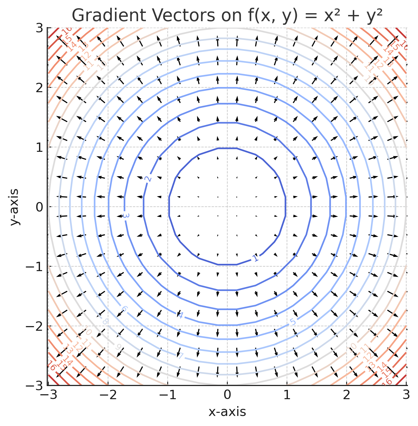
📊 Visualizing the Gradient
The gradient vector points in the direction of steepest increase of a function, and its magnitude tells you how steep the change is.
In a contour plot (like a topographic map), gradient vectors are always perpendicular to the level curves. Let’s visualize this with:
\[ f(x, y) = x^2 + y^2 \]
🔧 Python Code to Plot Gradient Vectors
1
2
3
4
5
6
7
8
9
10
11
12
13
14
15
16
17
18
19
20
21
22
23
import numpy as np
import matplotlib.pyplot as plt

# Create a mesh grid
X, Y = np.meshgrid(np.linspace(-3, 3, 20), np.linspace(-3, 3, 20))
Z = X**2 + Y**2


# Compute gradient components
U = 2 * X  # ∂f/∂x
V = 2 * Y  # ∂f/∂y

# Plot the contour and gradient vectors
plt.figure(figsize=(6, 6))
contours = plt.contour(X, Y, Z, levels=20, cmap='coolwarm')
plt.clabel(contours, inline=True, fontsize=8)
plt.quiver(X, Y, U, V, color='black')
plt.title('Gradient Vectors on f(x, y) = x² + y²')
plt.xlabel('x-axis')
plt.ylabel('y-axis')
plt.axis('equal')
plt.grid(True)
plt.show()
🤖 Why Gradients Matter in Machine Learning
Gradients aren’t just theoretical tools — they power the core of how machine learning models learn.
Here’s where gradients show up:
Gradient Descent
Gradients point in the direction of steepest increase, so we go in the opposite direction to minimize a loss function.
\[ \theta = \theta - \eta \cdot \nabla L(\theta) \] This simple update rule trains models like linear regression, logistic regression, and neural networks.Backpropagation (Neural Networks)
Partial derivatives are used to compute gradients of the loss with respect to each weight in the network. This helps propagate error backward and update parameters.Loss Function Optimization
Gradients tell us how sensitive the model’s output is to each parameter, which is key to reducing training error.Multivariable Models
In models with multiple inputs/features (e.g. \( f(x_1, x_2, \dots, x_n) \)), partial derivatives are essential for calculating how each feature affects predictions.
💡 Real-World Insight
If your model can’t compute gradients correctly, it can’t learn.
That’s why understanding the gradient — not just using it — gives you an edge when debugging training, tuning hyperparameters, or building custom architectures.
🚀 Level Up
- Gradients are more than just vectors — they guide optimization algorithms by pointing in the direction of steepest ascent.
- Gradient Descent works by moving opposite the gradient to minimize loss — it's the foundation of nearly all model training.
- Partial derivatives allow you to analyze how individual features affect a model's output — critical for explainability and debugging.
- Understanding gradients helps you implement custom training loops, fine-tune neural networks, and modify backpropagation rules.
- You’ll encounter gradients in tools like autograd, TensorFlow, and PyTorch — all of which automate partial derivative calculations behind the scenes.
✅ Best Practices
- ✅ Start with geometric intuition — visualize gradients as arrows pointing in the steepest direction.
- ✅ Treat all other variables as constants when computing a partial derivative — one variable at a time.
- ✅ Use symbolic math libraries (like
sympy) to verify gradient expressions step-by-step. - ✅ Practice computing gradients of simple scalar fields like \( f(x, y) = x^2 + y^2 \) before tackling loss functions.
- ✅ Relate the gradient vector back to machine learning tasks like gradient descent, backpropagation, and feature sensitivity.
⚠️ Common Pitfalls
- ❌ Forgetting to treat other variables as constants when computing partial derivatives.
- ❌ Confusing scalar derivatives with gradient vectors — gradients are multivariable vectors, not single numbers.
- ❌ Ignoring direction — the gradient not only gives magnitude but points in the direction of maximum increase.
- ❌ Reversing gradient direction in gradient descent — remember, you subtract the gradient to minimize.
- ❌ Skipping visualization — seeing the gradient field helps reveal structure that equations alone can hide.
📌 Try It Yourself
📊 What is the gradient of \( f(x, y) = x^2 + y^2 \)?
\[ \nabla f = \begin{bmatrix} 2x \\\\ 2y \end{bmatrix} \]📊 What is the gradient of \( f(x, y) = 3xy + y^2 \)?
\[ \frac{\partial f}{\partial x} = 3y, \quad \frac{\partial f}{\partial y} = 3x + 2y \] \[ \nabla f = \begin{bmatrix} 3y \\\\ 3x + 2y \end{bmatrix} \]📊 What is the gradient of \( f(x, y, z) = xyz \)?
\[ \frac{\partial f}{\partial x} = yz, \quad \frac{\partial f}{\partial y} = xz, \quad \frac{\partial f}{\partial z} = xy \] \[ \nabla f = \begin{bmatrix} yz \\\\ xz \\\\ xy \end{bmatrix} \]🔁 Summary: What You Learned
| Concept | Description |
|---|---|
| Partial Derivative | Rate of change w.r.t. one variable, holding others constant |
| Gradient Vector | Vector of all partial derivatives — shows direction and rate of steepest increase |
| Geometric Insight | Gradients are perpendicular to level curves in 2D, surfaces in 3D |
| Symbolic Gradient | Use tools like SymPy to compute gradients analytically |
| Contour Visualization | Helps you see how the gradient behaves spatially |
| ML Connection | Gradients power learning algorithms like gradient descent and backpropagation |
Understanding gradients prepares you to tackle the Chain Rule, Jacobian matrices, and the inner workings of learning in high-dimensional ML models.
🧭 Next Up:
In the next post, we’ll explore one of the most important tools in multivariable differentiation — the Chain Rule and Jacobian matrix.
You’ll learn:
- How the Chain Rule extends to functions with multiple variables
- What the Jacobian matrix represents and how to compute it
- How to handle composite functions and vector-valued functions
- Why Jacobians are essential for coordinate transformations, deep learning, and backpropagation
Get ready to climb deeper into the multivariable landscape — things are about to get multidimensional and matrix-powered!
📺 Explore the Channel

🎥 Hoda Osama AI
Learn statistics and machine learning concepts step by step with visuals and real examples.
💬 Got a Question?
Leave a comment or open an issue on GitHub — I love connecting with other learners and builders. 🔁