Understanding Z-Distribution and Using the Z-Table
Master the Z-distribution — a key concept in data science that transforms values into z-scores, enabling outlier detection, standardization, and easier comparison across datasets. Essential for statistics and machine learning.
📌 What is Z-Distribution?
The Z-distribution (standard normal distribution) is a powerful tool in statistics and machine learning used to standardize values and compare scores across different datasets. By converting raw data into z-scores, we can easily detect outliers, perform hypothesis testing, and interpret results on a common scale — centered at 0 with a standard deviation of 1.
📚 This post is part of the "Intro to Statistics" series
🔙 Previously: Understanding Normal Distribution
🔢 Why do we use Z-Distribution?
If you want to find the probability or the space far from the mean by any value (like 1.3), the Z-distribution helps by converting your values into a standardized form.
🔄 Converting Between X and Z
To work with any normal distribution, you first convert values \( X \) to their corresponding Z-scores:
\[ Z = \frac{X - \mu}{\sigma} \]
And vice versa:
\[ X = Z \times \sigma + \mu \]
📊 Understanding the Cumulative Z-Table
The Z-table (or standard normal table) shows the cumulative probability for the standard normal distribution \( Z \).
- It gives the probability that a standard normal variable \( Z \) is less than or equal to a given value.
- In other words, it shows the area under the curve to the left of a Z-score.
- Values in the table range from 0 to 1 because they represent probabilities.
How to Read the Z-Table
- Find the row corresponding to the first two digits and the first decimal place of your Z-score.
- Find the column corresponding to the second decimal place of your Z-score.
- The value where the row and column intersect is the cumulative probability.
For example, to find the cumulative probability for \( Z = 1.23 \):
- Look at the row for 1.2
- Look at the column for 0.03
- The table value at this intersection is approximately 0.8907
This means \( P(Z \leq 1.23) = 0.8907 \).
🧮 Example: Using the Z-Table
Suppose you want to find the probability that a standard normal variable \( Z \) is less than 1.23.
- Locate 1.2 in the rows.
- Locate 0.03 in the columns.
- The value in the table is 0.8907.
Thus, \( P(Z \leq 1.23) = 0.8907 \), meaning there is an 89.07% chance that \( Z \) is less than or equal to 1.23.
🔄 Summary of Using the Z-Table with Any Normal Distribution
- First, convert your \( X \) value to a Z-score using:
\[ Z = \frac{X - \mu}{\sigma} \]
- Then, use the Z-table to find the cumulative probability for that Z.
- If you want the probability between two values, find the cumulative probabilities for both and subtract the smaller from the larger.
📊 Visual Aid: Sample Z-Table (Partial)
| Z | .00 | .01 | .02 | .03 | .04 |
|---|---|---|---|---|---|
| 1.2 | 0.8849 | 0.8869 | 0.8888 | 0.8907 | 0.8925 |
| 1.3 | 0.9032 | 0.9049 | 0.9066 | 0.9082 | 0.9099 |
The value for Z=1.23 is highlighted.
🧮 Example: Finding Probability Between Two Values
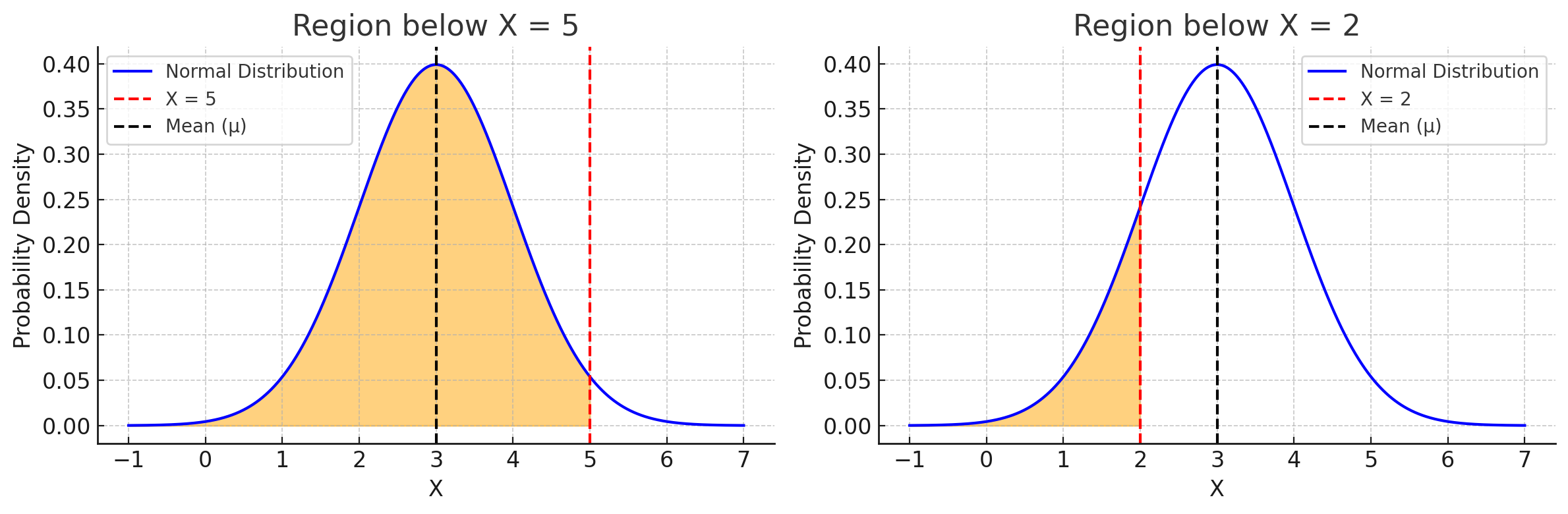
Suppose \( X \) is normally distributed with mean \( \mu = 3 \) and standard deviation \( \sigma = 1 \). We want to find the probability that \( X \) lies between 2 and 5.
Step 1: Convert \( X \) values to Z-scores
\[ Z = \frac{X - \mu}{\sigma} \]
Calculate:
\[ Z_1 = \frac{2 - 3}{1} = -1 \]
\[ Z_2 = \frac{5 - 3}{1} = 2 \]
Step 2: Find cumulative probabilities using the Z-table
- The cumulative probability for \( Z_2 = 2 \) is approximately 0.9772.
- The cumulative probability for \( Z_1 = -1 \) is approximately 0.1587.
Step 3: Subtract to get the probability between the two values
\[ P(2 < X < 5) = P(Z < 2) - P(Z < -1) = \] 0.9772 - 0.1587 = 0.8185
So, there is an approximately 81.85% chance that \( X \) lies between 2 and 5.
Visuals
Below are shaded regions representing these cumulative probabilities:
Area below \( X = 5 \):
Area below \( X = 2 \):
🔟 Example: 10th Percentile Duration
To find the 10th percentile, find the Z-score corresponding to 0.10 cumulative probability in the Z-table, then convert it back to \( X \):
\[ X = Z_{0.10} \times \sigma + \mu \]
🔄 Why Conversion Is Useful Beyond Normal Distributions
Converting \( X \) to \( Z \) can be applied to various data types and distributions, not just normal ones. It standardizes data for easier comparison and probability calculations.
🤖 Why It Matters for Machine Learning
- Z-scores are widely used to standardize features before feeding them into machine learning models like:
- Logistic Regression
- K-Nearest Neighbors (KNN)
- Support Vector Machines (SVM)
- Z-distribution helps with outlier detection — values with Z-scores beyond ±3 are often flagged as anomalies.
- Used in evaluating model performance with confidence intervals and hypothesis testing.
- Important for techniques assuming normality (e.g., Linear Regression, Naive Bayes, and PCA).
🧠 Level Up: Deep Dive into Z-Distribution
- The Z-distribution is a powerful tool for standardizing and comparing data across different normal distributions.
- It plays a key role in hypothesis testing, confidence interval calculation, and many inferential statistics methods.
- The cumulative distribution function (CDF) and its inverse (quantile function) allow us to compute probabilities and critical values.
- Learning to interpret Z-scores helps in identifying outliers and understanding data spread relative to the mean.
- Remember, the Z-table provides cumulative probabilities from the far left up to any Z-score, but you can also calculate tail probabilities for ranges beyond.
✅ Best Practices for Z-Distribution
- Always convert X to Z before using the Z-table.
- Use the Z-distribution for data that is approximately normal and standardized.
- Apply cumulative probabilities correctly: Z-table gives area to the left of Z.
- Use Z-scores to detect extreme values or outliers.
⚠️ Common Pitfalls
- ❌ Assuming the Z-distribution applies to non-normal data without verification.
- ❌ Reading the Z-table incorrectly (e.g., misreading Z = 1.23 as 1.32).
- ❌ Forgetting to standardize X before using the Z-table.
- ❌ Using Z-tables for right-tail probabilities without subtracting from 1.
📌 Try It Yourself: Z-Distribution
Q1: What are the mean and standard deviation of the standard normal (Z) distribution?
💡 Show Answer
Mean \( \mu = 0 \) and standard deviation \( \sigma = 1 \).
Q2: How do you convert a raw score \( X \) to a Z-score?
💡 Show Answer
\( Z = \frac{X - \mu}{\sigma} \)
Q3: What does the cumulative Z-table tell you?
💡 Show Answer
It gives the probability that the Z-score is less than or equal to a given value (area to the left of that Z).
Q4: How do you find the probability that \( X \) lies between two values?
💡 Show Answer
Convert both values to Z-scores, find their cumulative probabilities from the Z-table, and subtract the smaller from the larger.
Q5: What is the approximate probability that \( Z \) lies between -1 and 1?
💡 Show Answer
About 68% (using the empirical rule).
Bonus: How are Z-scores used in machine learning pipelines?
💡 Show Answer
✅ Z-scores standardize features, making them have mean = 0 and std dev = 1 — essential for many ML models like SVM, KNN, and logistic regression.
✅ Summary
| Concept | Description |
|---|---|
| Z-Distribution | Standard normal distribution with mean \( \mu=0 \), \( \sigma=1 \) |
| Z-Score | Measures how many standard deviations a value is from the mean: \( Z = \frac{X - \mu}{\sigma} \) |
| Cumulative Z-Table | Gives the probability \( P(Z \leq z) \), area under the curve to the left of \( z \) |
| Finding Probability Between Two Values | Convert \( X \) values to Z-scores, look up cumulative probabilities, subtract to find the probability between |
| Percentiles | Use Z-scores from the cumulative table and convert back to \( X \) values for interpretation |
🔜 Up Next
Next, we’ll explore the Binomial Distribution — a fundamental discrete distribution used to model the number of successes in a fixed number of independent trials.
Stay tuned!
📺 Explore the Channel

🎥 Hoda Osama AI
Learn statistics and machine learning concepts step by step with visuals and real examples.
💬 Got a Question?
Leave a comment or open an issue on GitHub — I love connecting with other learners and builders. 🔁