Z-Score: Comparing Values Using Standardization

Have you ever scored 90 on a test and wondered: Is that impressive or just average?
To answer that, you need more than just the number — you need to know how it compares to others. That’s exactly what a Z-score helps you do.

A Z-score tells you how far a value is from the mean in terms of standard deviations. It’s one of the most useful tools in statistics and machine learning for comparing values across different distributions, detecting outliers, and standardizing data for models.

In this post, you’ll learn what Z-scores are, how to calculate and interpret them, and how they’re used in real-world analysis.

---

📚 This post is part of the "Intro to Statistics" series

🔙 Previously: Measuring Variability: Variance and Standard Deviation

🔜 Next: Real Example: Putting It All Together

---

🎯 What is a Z-Score?

A Z-score (or standard score) tells you:

❓ “How many standard deviations is this value away from the mean?”

It answers:

• Is this value above or below average?
• Is it unusual or common in this distribution?

---

🤖 Why Z-Scores Matter in Machine Learning

Z-scores are used to:

• Standardize features (essential for models like KNN, SVM, logistic regression)
• Detect outliers in high-dimensional data
• Compare different variables on the same scale
• Improve feature scaling and model convergence

Z-scores make raw values comparable across features and distributions.

---

🧠 How Z score standardization fits into an ML pipeline

In machine learning, Z score standardization is usually applied as one step in the preprocessing pipeline.

The idea is:

1. Use the training data only to estimate:
   • Mean of each numeric feature \( \bar{x}_j \)
   • Standard deviation of each numeric feature \( s_j \)
2. Transform the training features: \[ z_{ij} = \frac{x_{ij} - \bar{x}_j}{s_j} \]
3. When you get validation or test data, use the same \( \bar{x}_j \) and \( s_j \) from the training set to transform them.

This is very important to avoid data leakage. If you compute the mean and standard deviation on the full dataset before splitting, information from the test set leaks into the training process.

In code, a typical pattern looks like:

# 1. Fit on training data
mu = X_train.mean(axis=0)
sigma = X_train.std(axis=0)

# 2. Transform training data
X_train_std = (X_train - mu) / sigma

# 3. Transform validation or test data with the same parameters
X_test_std = (X_test - mu) / sigma

---

⚖️ Z score vs other scaling methods

Z score standardization is not the only way to scale features. Here is how it compares to two common alternatives.

Method	Formula (idea)	Good for	Limitations
Z score	\( z = \dfrac{x - \bar{x}}{s} \)	Most numeric features that are roughly symmetric	Sensitive to strong outliers
Min max scaling	\( x’ = \dfrac{x - x_{\min}}{x_{\max} - x_{\min}} \)	Features that must stay in a fixed range such as [0, 1]	Very sensitive to extreme values
Robust scaling	\( x’ = \dfrac{x - \text{median}}{\text{IQR}} \)	Features with heavy outliers or very skewed data	Harder to interpret than Z scores

Practical guidance in ML:

• Use Z score standardization when features are numeric and not extremely skewed. It works well with KNN, SVM, linear and logistic regression, and neural networks.
• Use min max scaling when a model or activation function expects inputs in a bounded range, such as [0, 1] or [minus 1, 1]. This is common in some neural network setups and image processing.
• Use robust scaling when you have strong outliers that would distort the mean and standard deviation. It is useful before models that are sensitive to outliers.

The key idea is to choose a scaling method that matches the shape of your data and the requirements of your model, rather than applying Z score standardization automatically in every situation.

---

🚨 Using Z scores for outlier detection

Z scores are often used as a simple tool for spotting unusual values.

If the data are approximately normal:

• Values with \(|z| \le 2\) are usually considered typical
• Values with \(2 < |z| \le 3\) are possible outliers that deserve a closer look
• Values with \(|z| > 3\) are strong candidates for outliers

In practice:

• A large positive Z score means the value is far above the mean
• A large negative Z score means the value is far below the mean

Outliers in machine learning

In a machine learning context, you can use Z scores to:

• Detect suspicious data points that may be data entry errors
• Flag extreme values before training a model that is sensitive to outliers
• Decide whether to remove, cap, or transform extreme observations

Common strategies:

• Remove obvious data errors after verification

• Cap extreme Z scores at a chosen threshold (for example clip all values with (

  z

  > 3))

• Transform skewed features (for example with log or square root) before standardization

Important notes:

• Z score outlier rules work best when the distribution is roughly normal
• In high dimensional feature spaces, seeing some large Z scores is normal, so always combine Z scores with domain knowledge and plots instead of removing points blindly

---

🎯 Z scores, probabilities, and percentiles

When a variable is approximately normally distributed, Z scores connect directly to probabilities and percentiles.

From Z score to probability

If a standardized variable follows a standard normal distribution \( N(0, 1) \):

• A given Z score \( z \) tells you how far the value is from the mean in standard deviations
• The cumulative probability \( P(Z \le z) \) is the area under the curve to the left of \( z \)

Typical reference values:

• \( z = 0 \) → about 50 percent of values are below the mean
• \( z = 1 \) → about 84 percent of values are below
• \( z = 1.96 \) → about 97.5 percent of values are below
• \( z = 2 \) → about 97.7 percent of values are below

These probabilities come from the standard normal table or from statistical software.

Z scores and percentiles

A percentile tells you the percentage of observations that fall at or below a value.

• If a value has \( z = 0 \), it is at the 50th percentile
• If a value has \( z \approx 1.64 \), it is around the 95th percentile
• If a value has \( z \approx -1.64 \), it is around the 5th percentile

Example:

If exam scores are approximately normal and a student has \( z = 1.2 \), then their score is higher than about 89 percent of students. In other words, they are roughly at the 89th percentile.

Why this matters in ML

When model outputs or performance metrics are roughly normal, Z scores allow you to:

• Translate a raw value into a percentile (how extreme is this compared to typical behavior)
• Build approximate confidence intervals using cutoffs like \( z = 1.96 \) for 95 percent
• Compare how unusual different metrics are on a common scale

🧪 ML example: standardizing a feature before modeling

Imagine you are building a model to predict whether a patient has high cardiovascular risk using features like:

• Age (years)
• Systolic blood pressure (mmHg)
• Cholesterol level (mg/dL)

Suppose in your training data the cholesterol feature has:

• Sample mean \( \bar{x} = 200 \) mg/dL
• Sample standard deviation \( s = 40 \) mg/dL

For a new patient in the training set with cholesterol \( x = 260 \) mg/dL, the Z score is:

\[ z = \frac{x - \bar{x}}{s} = \frac{260 - 200}{40} = \frac{60}{40} = 1.5 \]

Interpretation:

• The patient’s cholesterol is 1.5 standard deviations above the training mean.
• In standardized form, the raw value 260 becomes a feature value of 1.5.

If you also standardize age and blood pressure, each feature will have:

• Mean close to 0
• Standard deviation close to 1

This helps many models, such as logistic regression, SVM, KNN, and neural networks, because:

• Features are on a comparable scale
• Gradient based optimization can converge more reliably
• Distance based models do not get dominated by features with large numeric ranges

---

🧪 ML example: standardizing a feature before modeling

Imagine you are building a model to predict whether a patient has high cardiovascular risk using features like:

• Age (years)
• Systolic blood pressure (mmHg)
• Cholesterol level (mg/dL)

Suppose in your training data the cholesterol feature has:

• Sample mean \( \bar{x} = 200 \) mg/dL
• Sample standard deviation \( s = 40 \) mg/dL

For a new patient in the training set with cholesterol \( x = 260 \) mg/dL, the Z score is:

\[ z = \frac{x - \bar{x}}{s} = \frac{260 - 200}{40} = \frac{60}{40} = 1.5 \]

Interpretation:

• The patient’s cholesterol is 1.5 standard deviations above the training mean.
• In standardized form, the raw value 260 becomes a feature value of 1.5.

If you also standardize age and blood pressure, each feature will have:

• Mean close to 0
• Standard deviation close to 1

This helps many models, such as logistic regression, SVM, KNN, and neural networks, because:

• Features are on a comparable scale
• Gradient based optimization can converge more reliably
• Distance based models do not get dominated by features with large numeric ranges

---

🧮 Z-Score Formula

\[ z = \frac{x - \bar{x}}{\sigma} \]

This formula transforms a raw score \( x \) into a standardized score:

• The numerator \( x - \bar{x} \) tells us how far the value is from the mean
• The denominator \( \sigma \) scales this difference using standard deviation
• The result is a unit-free number (z-score) showing its relative position

Where:

• \( x \): the observation
• \( \bar{x} \): the mean
• \( \sigma \): the standard deviation

(In practice, we usually use the sample standard deviation ( s ) computed from the data, as explained in the next section.)

---

📊 Population vs sample Z-scores

In theory, the Z-score is defined using the population mean and standard deviation:

\[ z = \frac{x - \mu}{\sigma} \]

In practice, we almost never know the population parameters, so we estimate them from a sample:

• Sample mean: \( \bar{x} \)
• Sample standard deviation: \( s \)

Then each Z-score is computed as:

\[ z_i = \frac{x_i - \bar{x}}{s} \]

Key idea:

• If you compute Z-scores for a dataset using its own sample mean \( \bar{x} \) and sample standard deviation \( s \), the positive and negative deviations balance and the Z-scores have:
  • Sum equal to zero
  • Mean equal to zero

In machine learning preprocessing, you are almost always using this sample based version. You estimate \( \bar{x} \) and \( s \) from your training data, then use those same values to standardize both training and test sets.

---

📊 Example: One Observation

Suppose:

• Mean = 70
• Standard Deviation = 10
• Observation = 85

Then:

\[ z = \frac{85 - 70}{10} = 1.5 \]

🟢 The value is 1.5 standard deviations above the mean.

Now try:

\[ z = \frac{60 - 70}{10} = -1 \]

🔵 This one is 1 standard deviation below the mean.

---

📈 How to Interpret Z-Scores

• Positive z-score → Above the mean
• Negative z-score → Below the mean
• z = 0 → Exactly the mean

Z-scores show where a value lies on the distribution curve.

📌 When the distribution is skewed:

• Right-skewed → Large z-scores occur more often in the tail
• Left-skewed → Negative z-scores dominate the lower tail

🔎 Important:
You can compute a Z-score for any numeric distribution, not only normal ones.

• When the data are approximately normal, Z-scores line up nicely with the empirical rule (about 68% within \(-1\) to \(+1\), 95% within \(-2\) to \(+2\), 99.7% within \(-3\) to \(+3\)).
• When the distribution is strongly skewed or has heavy tails, a Z-score still tells you how many standard deviations a value is from the mean, but the usual “unusual if \(|z| > 2\) or \(|z| > 3\)” rule might not match the true probabilities.

---

📉 Empirical Rules and Z-Score Ranges

There’s a general understanding of how much data falls in certain z-score ranges:

Z-Score Range	Approx. % of Data
-1 to +1	~68%
-2 to +2	~95%
-3 to +3	~99.7%

✅ So most values (especially in bell-shaped distributions) lie between -2 and +2.

---

🖼️ Visual Insight: Z-Scores and the Normal Distribution

The Z-score works best with normally distributed data. Here’s how the values are typically spread:

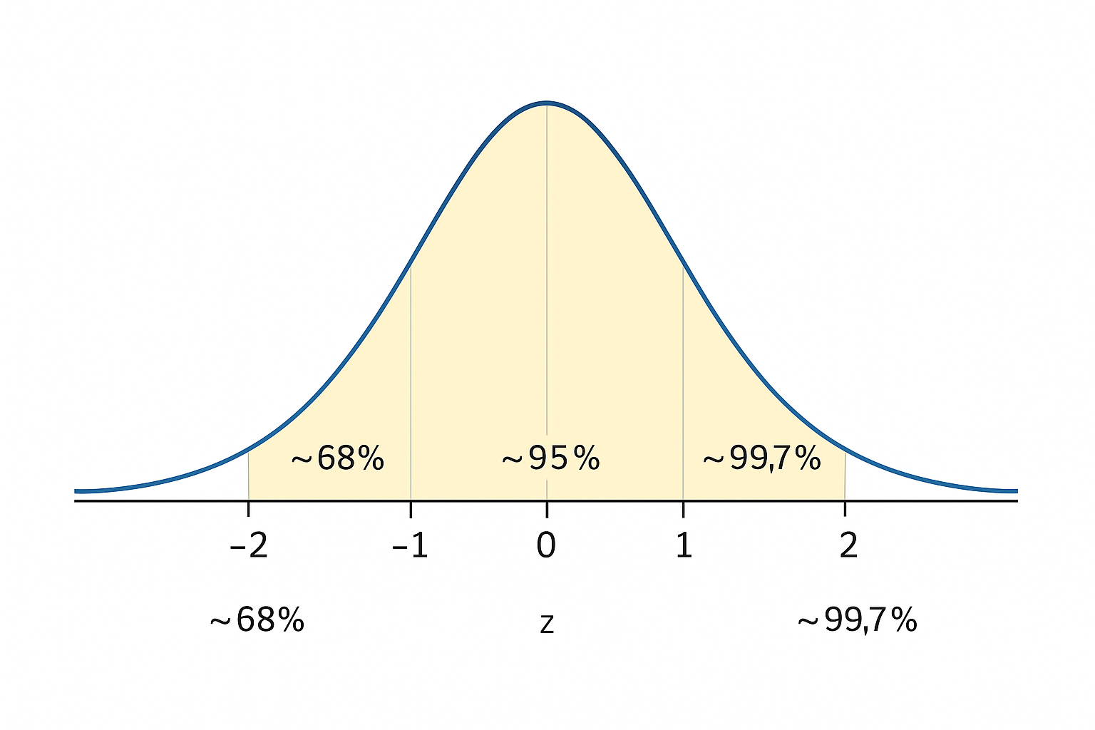
• ~68% of values fall between z = -1 and +1
• ~95% fall between z = -2 and +2
• ~99.7% fall between z = -3 and +3

✅ Use this to visually estimate how common or rare a value is based on its Z-score.

---

🔁 Z-Score Always Balances

If you compute z-scores for a dataset using its own sample mean and sample standard deviation, their sum is zero:

\[ \sum z = 0 \]

Here is the important detail:

• Suppose you have values \(x_1, x_2, \dots, x_n\) with sample mean \(\bar{x}\) and sample standard deviation \(s\).
• If you define each z-score as \(z_i = \dfrac{x_i - \bar{x}}{s}\), then the positive and negative deviations cancel and \(\sum_{i=1}^{n} z_i = 0\).
• If you use any other mean or standard deviation (for example population values or parameters from another dataset), the sum of z-scores will not usually be zero.

---

🧪 Multiple Z-Scores from a Dataset

Let’s say we have a dataset of exam scores:
{70, 80, 90}

Step 1 — Find the mean and standard deviation:

• Mean = \( \bar{x} = 80 \)
• Sample standard deviation =
  \[ s = \sqrt{\frac{(70-80)^2 + (80-80)^2 + (90-80)^2}{3 - 1}} = \sqrt{\frac{100 + 0 + 100}{2}} = \sqrt{100} = 10 \]

Step 2 — Compute z-scores for each value:

\[ z_{70} = \frac{70 - 80}{10} = -1 \]

\[ z_{80} = \frac{80 - 80}{10} = 0 \]

\[ z_{90} = \frac{90 - 80}{10} = 1 \]

These scores tell us:

• 70 is below average
• 80 is exactly the average
• 90 is above average

✅ The sum of these z-scores ≈ 0, confirming the rule.

---

⚖️ Comparing Across Distributions

Let’s say we have two distributions:

Test A:

• Mean = 60, SD = 5
• Observation = 70
  \[ z = \frac{70 - 60}{5} = 2 \]

Test B:

• Mean = 85, SD = 10
• Observation = 90
  \[ z = \frac{90 - 85}{10} = 0.5 \]

📌 Although 90 is numerically higher, it is less exceptional in Test B than 70 is in Test A.

---

🌍 This is Called Standardization

Standardization means:

Expressing a value in terms of how far it is from the mean, using the standard deviation.

It lets us:

• Compare scores from different tests
• Identify outliers
• Normalize data for machine learning

---

✅ Best practices when using Z scores

• Standardize numeric features for sensitive models. Use Z score standardization for models that rely on distances or gradients, such as KNN, SVM, linear and logistic regression, and neural networks.
• Fit scaling on the training set only. Always compute the mean and standard deviation using the training data, then apply those same parameters to validation and test sets to avoid data leakage.
• Inspect distributions before scaling. Look at histograms or summary statistics to see if features are roughly symmetric or heavily skewed before deciding how to scale them.
• Use Z scores to compare different variables. When features are on very different scales, convert them to Z scores to compare how extreme an individual value is across variables.
• Combine Z scores with domain knowledge. Treat unusually large or small Z scores as signals to investigate, not automatic reasons to delete data.

---

⚠️ Common pitfalls with Z scores

• Computing Z scores on the full dataset before splitting. This leaks information from the test set into the training process and can give overly optimistic performance estimates.
• Interpreting Z as probability. A Z score is a distance in standard deviation units, not a probability. Probabilities come from the normal distribution using that Z value.
• Assuming normality when the data are strongly skewed. The usual ideas about typical and unusual Z scores (like 68, 95, 99.7 percent) only hold well when the distribution is close to normal.
• Applying Z scores to inappropriate variables. Do not standardize arbitrary category codes or identifiers where numeric distances have no real meaning.
• Removing all points with large Z scores automatically. Many real data sets naturally contain extreme but valid values. Always check context before dropping or capping them.

---

🧠 Level Up: How Z-Scores Power Real Analysis

Z-scores are useful not just for detecting outliers or comparing scores, but also in **statistical inference** and **ML pipelines**. Here's how they're used in real-world applications:

• 🎯 Probability: Z-scores help us estimate how likely a value is in a normal distribution — using z-tables
• 📏 Confidence Intervals: Z-scores define the range of values we expect sample means to fall within
• 🚨 Outlier Detection: Observations with |z| > 2 or |z| > 3 are often flagged as potential outliers
• 🔄 Standardization: Machine learning models often require data to be normalized using z-scores

You’ll see these ideas come to life as we explore probability and inference in upcoming posts.

---

📌 Try It Yourself

Q: A student received a test score with a z-score of -2.1. What does this tell you about the score compared to the rest of the class?

💡 Show Answer

✅ It means the score is 2.1 standard deviations below the mean — significantly lower than average. In most distributions, that would place the score in the bottom 2%–3% of the group.

---

🧠 Summary

Concept	What It Means	Practical Use
Z-score	Distance from mean in standard deviations	Normalization, outlier detection
Positive z	Above average	High-performing observation
Negative z	Below average	Underperformance or anomaly
z = 0	Exactly average	Benchmark reference point
Sum of all z	Zero when using the dataset’s own mean and standard deviation	Confirms correct standardization on that dataset

---

💬 Have a question or want to compare z-scores from your own dataset?
Drop it in the comments — happy to help!

---

✅ Up Next

Next, we’ll walk through a real-life example that uses everything we’ve learned:

• Mean
• Median
• Standard deviation
• Z-scores
  And how to interpret and compare them together.

Stay tuned!